Sensitivity and Uncertainty Analyses: Training Module
PDF version of this training | All modeling training modules
Sensitivity and Uncertainty Analyses
This module builds upon the fundamental concepts outlined in previous modules: Environmental Modeling 101 and Best Modeling Practices: Model Evaluation. The purpose of this module is to provide extended guidance on the concepts of sensitivity and uncertainty analyses - not to provide thorough instruction on the available methods or practices. When appropriate, this module will point the user in the direction of technical guidance.
Uncertainty Analysis - Investigates the effects of lack of knowledge or potential errors of the model (e.g. the uncertainty associated with parameter values or model design and output).
Sensitivity Analysis - The computation of the effect of changes in input values or assumptions (including boundaries and model functional form) on the outputs.
Uncertainty and sensitivity analysis are an integral part of the modeling process (Saltelli et al., 2000).

This module will expand upon the topics discussed in the Guidance Document (EPA, 2009a). Available for download.
The Process of Model Evaluation
Model evaluation is defined as the process used to generate information that will determine whether a model and its analytical results are of a sufficient quality to inform a decision (EPA, 2009a).
In practice, model evaluation should occur throughout the model's life-cycle.
Model Life-cycle:
The processes included when taking the conceptual understandings of an environmental process to a full analytical model is called the model life-cycle. The life-cycle is broken down into four stages: identification, development, evaluation, and application. Similarly, the NRC (2007) has also identified elements of model evaluation.
For review, the recommended practices associated with model evaluation include (EPA, 2009a):
- Peer Review
 Peer ReviewA documented critical review of work by qualified individuals (or organizations)who are independent of those who performed the work, but are collectively equivalent in technical expertise. A peer review is conducted to ensure that activities are technically adequate, competently performed, properly documented, and satisfy established technical and quality requirements. The peer review is an in-depth assessment of the assumptions, calculations, extrapolations, alternate interpretations, methodology, acceptance criteria, and conclusions pertaining to specific work and of the documentation that supports them.
 - Corroboration
- Quality Assurance (QA) and Quality Control (QC)
- Sensitivity Analysis
- Uncertainty Analysis
![]()
Additional Web Resources:
Further information can be found in these modules:
Model Corroboration
Model corroboration assesses the degree to which a model corresponds to reality, using both quantitative and qualitative methods. The modelers may use a graded approach to determine the rigor of these assessments which should be appropriately defined for each model application.
Qualitative methods, like expert elicitation![]() expert elicitationA systematic process for quantifying, typically in probabilistic terms, expert judgments about uncertain quantities. Expert elicitation may be used to characterize uncertainty and fill data gaps where traditional scientific research is not feasible or data are not yet available. Typically, the necessary quantities are obtained through structured interviews and/or questionnaires. Procedural steps can be used to minimize the effects of heuristics and bias in expert judgments., can provide the development team with beliefs about a system's behavior in a data-poor situation. Utilizing the expert knowledge available, qualitative corroboration is achieved through consensus and consistency (EPA, 2009a).
expert elicitationA systematic process for quantifying, typically in probabilistic terms, expert judgments about uncertain quantities. Expert elicitation may be used to characterize uncertainty and fill data gaps where traditional scientific research is not feasible or data are not yet available. Typically, the necessary quantities are obtained through structured interviews and/or questionnaires. Procedural steps can be used to minimize the effects of heuristics and bias in expert judgments., can provide the development team with beliefs about a system's behavior in a data-poor situation. Utilizing the expert knowledge available, qualitative corroboration is achieved through consensus and consistency (EPA, 2009a).
QA Planning and Data Quality Assessment
A well-executed quality assurance project plan (QAPP) helps to ensure that a model performs the specified task. The objectives and specifications of the model set forth in a quality assurance plan can be subjected to peer review.
Data quality assessments are an integral component of any QA plan that includes modeling activities. Similar to peer review, data quality assessments evaluate and assure that (EPA, 2002a):
- the data used by the model is of high quality
- data uncertainty is minimized
- the model has a foundation of sound scientific principles
![]()
Additional Web Resource:
Additional information on QA planning (including guidance documents) can be found at the Agency’s website for the Quality System for Environmental Data and Technology.
NRC (2007) defined elements of model evaluation:
- Evaluation of the scientific basis of the model
- Computational infrastructure
- Assumptions and limitations
- Peer review
- QA/QC controls and measures
- Data availability and quality
- Test cases
- Corroboration of model results with observations
- Benchmarking against other models
- Sensitivity and Uncertainty Analyses
- Model resolution capabilities
- Degree of transparency
Variability
The CREM Guidance Document (EPA, 2009a) uses the term "data uncertainty" to refer to the uncertainty caused by measurement errors, analytical imprecision and limited sample sizes during data collection and treatment.
In contrast to data uncertainty, variability results from the inherent randomness of certain parameters or measured data, which in turn results from the heterogeneity and diversity in environmental processes (EPA, 1997). Variability can be better characterized, but hard to reduce, with further study.
Separating variability and uncertainty is necessary to provide greater accountability and transparency (EPA, 1997). However, variability and uncertainty are inextricably intertwined and ever present in regulatory decision making (EPA, 2001a; 2003).
Uncertainty
In the general sense, uncertainty can be discussed in terms of its nature and type. Alternatively, uncertainty can also be discussed in terms of its reducibility or lack thereof (see Mattot et al., 2009).
Uncertainty is present and inherent throughout the modeling process and within a modeling context is termed model uncertainty. Model uncertainty arises from a lack of knowledge about natural processes, mathematical formulations and associated parameters![]() parametersTerms in the model that are fixed during a model run or simulation but can be changed in different runs as a method for conducting sensitivity analysis or to achieve calibration goals., and/or data coverage and quality. Walker et al. (2003) identify yet another model uncertainty assigned to the predicted output of the model.
parametersTerms in the model that are fixed during a model run or simulation but can be changed in different runs as a method for conducting sensitivity analysis or to achieve calibration goals., and/or data coverage and quality. Walker et al. (2003) identify yet another model uncertainty assigned to the predicted output of the model.
Despite these uncertainties, models can continue to be valuable tools for informing decisions through proper evaluation and communication of the associated uncertainties (EPA, 2009a).
Uncertainty analysis (UA) investigates the effects of lack of knowledge or potential errors on model output. When UA is conducted in combination with sensitivity analysis; the model user can become more informed about the model user can become more informed about the confidence that can be placed in model results (EPA, 2009a).
Nature of Uncertainty:
The nature of uncertainty can be described as (Walker et al., 2003; Pascual 2005; EPA, 2009b):
- Stochastic uncertainty - resulting from errors in empirical measurements or from the world's inherent stochasticity "Variability-related uncertainty"
- Epistemic uncertainty - uncertainty from imperfect knowledge (of the system being modeled) "Knowledge-related uncertainty"
- Technical uncertainty - uncertainty associated with calculation errors, insufficient data, numerical approximations, and errors in the model or computational algorithms
Type of Uncertainty:
Total uncertainty (in a modeling context) is the combination of many types of uncertainty (Hanna, 1988; EPA, 1997; 2003, Walker et al., 2003):
- Data/input uncertainty - variability, measurement errors, sampling errors, systematic errors
- In some conventions, parameter uncertainty, is discussed separately. This type of uncertainty is assigned to the data used to calibrate parameter values
- Model uncertainty - simplification of real-world processes, mis-specification of the model structure, use of inappropriate variable or parameter values, aggregation errors, application/scenario
Model Uncertainty
EPA (2009a) identifies uncertainties that affect model quality.
- Application niche uncertainty - uncertainty attributed to the appropriateness of a model for use under a specific set of conditions (i.e. a model application scenario). Also called 'scenario uncertainty'.
- Structure/framework uncertainty - incomplete knowledge about factors that control the behavior of the system being modeled; limitations in spatial or temporal resolution; and simplifications of the system.
- Parameter uncertainty - resulting from data measurement errors; inconsistencies between measured values and those used by the model.
Model Complexity and Uncertainty
The relationship between model uncertainty and model complexity is important to consider during model development. Increasingly complex models have reduced model framework/theory uncertainty as more scientific understandings are incorporated into the model. However, as models become more complex by including additional physical, chemical, or biological processes, their performance can degrade because they require more input variables, leading to greater data uncertainty (EPA, 2009a).
An NRC Committee (2007) recommended that models used in the regulatory process should be no more complicated than is necessary to inform regulatory decision and that it is often preferable to omit capabilities that do not substantially improve model performance.

Relationship between model framework uncertainty and data uncertainty, and their combined effect on total model uncertainty. Application niche uncertainty would scale the total uncertainty. Adapted from Hanna (1988) and EPA (2009a).
A Summary of Model and Data Uncertainty
| Model Uncertainty | Data/Input Uncertainty | ||||
|---|---|---|---|---|---|
| Application Niche | Structural / Framework | Parameter | Systematic / Measurement Error | Variability and Random Error | |
| Nature | Knowledge related | Knowledge related | Knowledge and Variability related | N/A | Variability related |
| Qualitative or Quantitative | Qualitative | Qualitative | Quantitative | Quantitative | Quantitative |
| Reducible | Yes | Yes | Yes | Yes – but always present | Can be better characterized, but not eliminated |
| Method to Characterize | Expert Elicitation; Peer Review | Expert Elicitation; Peer Review | Basic statistical measures | Bias | Basic statistical measures |
| How to Resolve | Appropriate application of model | Better scientific understanding; determining appropriate level of model complexity | Better scientific understanding; more data supporting the value | Improved measurements | More sampling |
Sensitivity Analysis
Sensitivity analysis (SA) is a method to determine which variables, parameters, or other inputs have the most influence on the model output. Sensitivity analyses are not 'pass / fail' evaluations, but rather informative analyses.
There can be two purposes for conducting a sensitivity analysis:
- SA computes the effect of changes in model inputs on the outputs.
- SA can be used to study how uncertainty in a model output can be systematically apportioned to different sources of uncertainty in the model input.**
**By definition, this second function of sensitivity analysis is a special case of uncertainty analysis.

A spider diagram used to compare relative changes in model output to relative changes in the parameter values can reveal sensitivities for each parameter (Addiscott, 1993). In this example, the effects of changing parameters A, B, and C are compared to relative changes in model output. The legs represent the extent and direction of the effects of changing parameter values.
Methods of Sensitivity Analysis
There are many methods for sensitivity analysis (SA), a few of which were highlighted in the Guidance on the Development, Evaluation, and Application of Environmental Models (EPA, 2009a). The chosen method should be agreed upon during model development and consider the amount and type of information needed from the analysis. Those methods are categorized into:
- Screening Tools
- Parametric Sensitivity Analyses
- Monte Carlo Analysis
- Differential Analysis Methods
Depending on underlying assumptions of the model, it may be best to start SA with simple methods to identify the most sensitive inputs and then apply more intensive methods to those inputs. A thorough review of methods can be found in Frey and Patil (2002).
Screening Tools
Preliminary screening tools are used instead of more intensive methods that involve multiple model simulations (Cullen and Frey, 1999; EPA, 2009a). By identifying parameters that have major influence on model output, you can focus further analyses on those parameters. Examples of screening tools:
Descriptive statistics: Select summary statistics (Coefficient of variation, Gaussian approximations, etc.) can be used to indicate the proportionate contribution of input uncertainties.
Scatter plots: A high correlation between an input and output variable may indicate dependence of the output variation on the, variation of the input.
Pearson’s Correlation Coefficient (ρ): Reflects the relationship between two variables. It ranges from (+1) to (-1). A correlation (ρ) of (+1) or (-1) means that there is a perfect positive or negative linear relationship between variables, respectively.
Terminology for Sensitivity Analysis
For many of the methods it is important to consider the geometry of the response plane and potential interactions or dependencies among parameters and/or input variables.
Response Surface/Plane: A theoretical multi-dimensional 'surface' that describes the response of a model to changes in input values. A response surface is also known as a sensitivity surface.
- Local Sensitivity Analysis: analysis conducted in close proximity to a nominal point of a response surface (i.e. works intensely around a specific set of input values) (EPA, 2003).
- Global Sensitivity Analysis: analysis across the entire response surface. Global sensitivity analysis can be of use as a quality assurance tool, to make sure that the assumed dependence of the output on the input factors in the model makes physical sense and represents the scientific understanding of the system (Saltelli et al., 2000).
Local Sensitivity Analysis
A response surface for a local sensitivity analysis. Here, the model output (y) is a function of (X1) and (X2). In a local sensitivity analysis, one often assumes a simple (i.e. linear) response surface over an appropriate interval of X1 and X2. Figure was adapted from EPA (2009a).

Global Sensitivity Analysis
A response surface for the function (Y) with parameters X1 and X2. For global sensitivity analyses, it is apparent that assumptions at the local scale (magnified area) may not hold true at the global scale. Complex (non-linear) functions and interactions among variables and parameters change the shape of the response surface. Figure was adapted from EPA (2009a).
 with parameters X1 and X2.")
Parametric Sensitivity Analysis
Parametric sensitivity analysis is a very common method which provides a measure of the influence input factors (data or parameters) have on model output variation. It does not quantify the effects of interactions because input factors are analyzed individually. However, this approach can indicate the presence of interactions.
A base case of model input values are set and then for each model run (simulation) a single input variable or parameter of interest is adjusted by a given amount, holding all other inputs and parameters constant (sometimes called "one-at-a-time").
A non-intensive sensitivity analysis can first be applied to identify the most sensitive inputs. By discovering the 'relative sensitivity' of model parameters, the model development team is then aware of the relative importance of parameters in the model and can select a subset of the inputs for more rigorous sensitivity analyses (EPA, 2009a). This also ensures that a single parameter is not overly influencing the results. This approach is considered non-intensive, in that it can be automated in some instances.
An example of a parametric sensitivity analysis is given on the Example subtab in this section.

An example of non-intensive sensitivity analysis. Relative sensitivities ofF (model output) with respect to parameters a and b. In this example, it is clear that parameter a has little influence on the model output, F; however, parameter b, has an interesting effect on model output, F. Adapted from EPA (2002b).
Monte Carlo Analysis
Monte Carlo simulations are based on repeated sampling and are a popular way to incorporate the variance of the input factors (e.g. parameter values or data) on the model output. Depending on the work and time needed to run the model, Monte Carlo simulations (often 1000's of iterations) can be difficult to impossible.
Overview of a Monte Carlo simulation:
- Randomly draw a value for each parameter of interest from an appropriate distribution. Note that the multiple parameters can be analyzed simultaneously.
- Run the model to make a prediction using the selected set of parameters
- Store prediction
- Repeat MANY times
- Analyze the distribution of predictions
More examples of Monte Carlo simulations appear in the next section under Quantitative Methods.

This figure is an example of the Monte Carlo simulation method. The distribution of internal concentration (model output) versus time is simulated by repeatedly (often as many as 10,000 iterations) sampling input values based on the distributions of individual parameters (blood flow rate, body weight, metabolic enzymes, partition coefficients, etc.) from a population. Adapted from EPA (2006).
Differential Analysis
Differential analyses typically contain four steps. Again, depending on the work and time needed to run the model, this approach can be difficult to impossible.
Four steps of a differential analysis (Saltelli et al., 2000; EPA, 2009a):
- Select base values and ranges for input factors.
- Using the input base values, develop a Taylor series approximation to the output.
- Estimate uncertainty of the output in terms of its expected value and variance using variance propagation techniques.
- Use the Taylor series approximations to estimate the importance of individual input factors.
The assumptions for differential sensitivity analysis include (EPA, 2009a):
- The model's response surface is hyperplane
- The results of a sensitivity analysis only apply to specific points on the response surface and that these points are monotonic first order
- Interactions among input variables are ignored
Further Insight
Computational methods for this technique are described in: Morgan, G., and M. Henrion. 1990. Uncertainty: A Guide to Dealing With Uncertainty in Quantitative Risk and Policy Analysis. Cambridge, U.K.: Cambridge University Press.
Parametric Analysis of the Markal Model
MARKAL is a data-intensive, technology-rich, energy systems economic optimization model that consists of two parts:
- an energy-economic optimization framework
- a large database that contains the structure and attributes of the energy system being modeled.
An illustrative example of a sensitivity analysis of MARKAL to examine the penetration of hydrogen fuel cell vehicles into the light-duty vehicle fleet is tracked (Y-axis) as model output. The reference case level of hydrogen fuel cell vehicle penetration in 2030 is 0%. This is represented by the point at the origin. The magnitude of each input is increased and decreased parametrically along a range deemed realistic for real-world values. The figure shows, for example, that a 25% increase in gasoline and diesel cost results in a model-predicted hydrogen fuel cell vehicle penetration of approximately 12%. Increasing the cost of gasoline and diesel by 50% increases penetration to around 25%. The analysis conveys a great deal of information, including not only the maximum magnitude of the response but also the response threshold and an empirical function of that response.
(Note: Results shown are for illustrative purposes only)
 Sensitivity diagram in which five inputs to the MARKAL model are changed parametrically and the response of an output is tracked. Note: Results shown above are for illustrative purposes only.
The inputs evaluated in this parametric sensitivity analysis include:
- the cost of gasoline and diesel fuel
- the cost of gasoline hybrid-electric vehicles (Gasoline-HEVcost)
- the cost of hydrogen fuel cell vehicles (H-FCVcost)
- the efficiency of gasoline hybrid electric vehicles (Gasoline-HEV efficiency)
- the cost of H2 fuel.
![]()
Additional Web Resources:
Additional information on the MARKet Allocation (MARKAL) model:
Uncertainty Analysis
The end goal of an uncertainty analysis may be to examine and report the sources and level of uncertainty associated with the modeling results. The level of uncertainty should meet the criteria determined at the onset of the modeling activity. This information can also help to identify areas that may need more research to reduce the associated uncertainty.
Some uncertainties can be quantified (e.g. data/input, parameter, and model output); whereas other uncertainties are better characterized qualitatively (e.g. model framework and the underlying theory or model application). Therefore, uncertainty analysis is presented in both quantitative and qualitative approaches.
Questions to consider before an uncertainty analysis:
- What is the objective of the uncertainty analysis?
- Who are the results (and uncertainties) going to be communicated to?
- What level of uncertainty is acceptable for the end decision?
- What resources are available to conduct the uncertainty analysis?
Further Insight:
EPA (2003) defined two categories of uncertainty analysis: compositional and performance. These categorizations are important to consider but extend beyond the scope of this module. For more information please see:
Multimedia, Multipathway, and Multireceptor Risk Assessment (3MRA) Modeling System Volume IV: Evaluating Uncertainty and Sensitivity. 2003. EPA530-D-03-001d. Office of Research and Development. US Environmental Protection Agency.
Prioritizing Uncertainty Reduction
Though some of the uncertainties presented in this module are unavoidable; peer review and practices to increase transparency![]() transparencyThe clarity and completeness with which data, assumptions and methods of analysis are documented. Experimental replication is possible when information about modeling processes is properly and adequately communicated. should help to better characterize them. Some uncertainties are easier to reduce than others. Recall that model uncertainty is comprised of:
transparencyThe clarity and completeness with which data, assumptions and methods of analysis are documented. Experimental replication is possible when information about modeling processes is properly and adequately communicated. should help to better characterize them. Some uncertainties are easier to reduce than others. Recall that model uncertainty is comprised of:
- Application niche uncertainty
- Parameter uncertainty
- Structural / Framework uncertainty
The application niche determines the set of conditions under which use of the model is scientifically defensible (EPA, 2009a). Therefore, application niche uncertainty can be minimized when the model is applied as intended.
Uncertainty analyses should be prioritized and conducted to characterize the uncertainty in a transparent way that is suited to the needs of the model application (e.g. decision-making informed by model results). This module will also explore tiered approaches to uncertainty analysis with the understanding that uncertainty analysis does not have a one-size-fits-all approach/method.
Efforts to characterize model uncertainties should focus upon (EPA, 2009a):
- Mapping the model attributes to the problem statement
- Confirming the degree of certainty needed from model outputs
- Determining the amount of reliable data available or the resources available to collect more
- The quality of the scientific foundations of the model
- The technical competence of the model development / application team
Quantitative Methods of Uncertainty Analysis
The WHO (2008) presented three levels of quantitative uncertainty analysis; briefly summarized here. These levels of uncertainty analysis correspond to the tiered approaches (discussed later in this section) presented with detailed examples.
Quantifying Variability
When only variability is quantified, the output is a single distribution representing a 'best estimate' of variation in the model output.
This approach can be used to make estimates for different percentiles of the distribution, but provides no confidence intervals; which may lead to a false impression of certainty (WHO, 2008).
1D Monte Carlo
Inputs (e.g. parameteres or data) to the model have distributions that represent both variability and uncertainty. These input distributions are combined in the output as a single distribution representing a mixture of variability and uncertainty.
This approach can be interpreted as an uncertainty distribution for the exposure of a single member of the population selected at random (i.e."the probability of a randomly chosen individual being exposed to any given level")
2D Monte Carlo
Is similar to the 1D approach, but instead, variability and uncertainty are propagated in the model and shown separately in the output.
For example, the output is typically presented as three cumulative curves: a central one representing the median estimate of the distribution for variation in exposure, and two outer ones representing lower and upper confidence bounds for the distribution.
Interpreted as: "Exposure estimates for different percentiles of the population, together with confidence bounds showing the combined effect of those uncertainties".
Approach Comparison
Comparison between three alternative probabilistic approaches for the same exposure assessment. In option 1, only variability is quantified (dotted blue line). In option 2, both variability and uncertainty are propagatedtogether (solid green line). In option 3, variability and uncertainty are propagated separately [dashed (uncertainty) and solid (variability) black line]. MC = Monte Carlo. 1D = one dimensional; ]. 2D = two dimensional. Image adapted from WHO (2008). (Click on image for a larger version)
![]()
Additional Web Resource:
For further information about exposure modeling please see: Human Exposure Modeling General Information

Qualitative Approaches to Uncertainty Analysis
In a qualitative uncertainty analysis, a description of the uncertainty in each of the major elements of the analysis is provided. Often, a statement of the estimated magnitude of the uncertainty (e.g. small, medium, large) and the impact the uncertainty might have on the outcome is included (EPA, 2004). Other components of qualitative uncertainty analysis can include (WHO, 2008):
- Qualitatively evaluate the level of uncertainty of each specified uncertainty (model, data, stochastic, etc.)
- Define the major sources of uncertainty
- Qualitatively evaluate the appraisal of the knowledge base of each major source
- Determine the controversial sources of uncertainty
- Qualitatively evaluate the subjectivity of choices of each controversial source
- Reiterate this methodology until the output satisfies predetermined objectives defined during model development (see EPA, 2009a).
- A Case Study of a qualitative uncertainty analysis from EPA's Region 8.
Level of Uncertainty
A scale of uncertainty from determinism to complete ignorance. Adapted from Walker et al. (2003).
The level of uncertainty can be the assessor's description of the degree of severity of the uncertainty. This scale ranges from "low" levels (determinism) to "high" levels (ignorance) - as depicted in the image (Walker et al., 2003; WHO, 2008).

Appraisal of the Knowledge Base:
This analysis focuses on how well the available data meet the needs of the modeling activity. These needs should have been identified during model development (EPA, 2009a). Examples of criteria for qualitatively evaluating the uncertainty of the knowledge base are adapted below from WHO (2008):
- AccuracyAccuracyCloseness of a measured or computed value to its "true" value, where the "true" value is obtained with perfect information. Due to the natural heterogeneity and stochasticity of many environmental systems, this "true" value exists as a distribution rather than a discrete value. In these cases, the "true" value will be a function of spatial and temporal aggregation.
- ReliabilityReliabilityThe confidence that (potential) users have in a model and in the information derived from the model such that they are willing to use the model and the derived information. Specifically, reliability is a function of the performance record of a model and its conformance to best available, practicable science.
- PlausibilityPlausibilityThe degree to which a cause-effect relationship would be expected, given known facts.
- Scientific consistency
- Robustness
A Modeling Caveat
The EPA recommends using the terms 'precision' and 'bias,' rather than 'accuracy,' to convey the information usually associated with accuracy.
Subjectivity of Choices:
This analysis provides insight into the choice processes for making assumptions during model development or application. EPA (2009a) recommends documenting these decisions and assumptions during model development.
Examples of criteria for evaluating the subjectivity of choices are adapted below from WHO (2008):
- Intersubjectivity among peers and among stakeholders
- Influence of situational/organization constraints on the choices
- Sensitivity of choices to the analysts' interests
- Influence of choices on results
Example
An example of a qualitative summary of uncertainties in the Baseline Ecological Risk Assessment (EPA, 2005).
| Assessment Component | Uncertainty Description | Likely Direction of Error | Likely Magnitude of Error |
|---|---|---|---|
| Exposure Assessment | Some exposure pathways were not evaluated. | Underestimate of Risk | Unknown, could be significant |
| Some chemicals were not evaluated because chemical was never detected, but detection limit was too high to detect the chemical if it were present at a level of concern. | Underestimate of Risk | Usually small | |
| Exposure point concentrations for wildlife receptors based on a limited measured dataset. | Use of upperc confidence level or max detect is likely to overestimate risk | Variable, can be evaluated by comparing best estimate to upper bound estimate | |
| Exposure parameters for wildlife receptors are based on studies at other sites. | Unknown | Probably small | |
| Absorption from site media is assumed to be the same as in laboratory studies. | Overestimate of risks | Probably significant |
Further Insight
Excerpt from Baseline Ecological Risk Assessment for the International Smelting & Refining Site, Tooele County, Utah, January 2005
Tiered Approaches to Uncertainty Analysis
The process for identifying the important sources of variability and uncertainty in a model's output is difficult. Therefore, tiered approaches are used to determine the appropriate level of analysis that is consistent with the objectives, the data available, and the information that is needed to inform a decision (EPA, 1997; 2001b).
Different techniques can be used in each of the tiers: see the tiered process for probabilistic risk assessment (WHO, 2008; EPA, 2009b); or the tiered approach outlined in EPA (2001b, 2004) described below:
- Tier 1 - Screening Level: point estimate sensitivity analysis (e.g. parametric sensitivity analysis, sensitivity ratios, etc.); simple, screening-level analyses using conservative assumptions and relatively simple modeling
- Tier 2 - Moderate Complexity: Probabilistic analyses. This combines uncertainty and variability information (e.g. 1D Monte Carlo)
- Tier 3 - High Complexity: Probabilistic sensitivity analyses, Bayesian analyses. Uncertainty and variability are distinguished from one another in the model output (e.g. 2D Monte Carlo).
 A schematic of a tiered approach. Image adapted from EPA (2001b; 2004).
Also recall the figure from WHO (2008) that depicts three approaches to uncertainty analysis.
Tier 2 - Moderate Complexity
An example comes from the Atmospheric Modeling and Analysis Division (AMAD) of the EPA's Office of Research and Development. In this example, the CMAQ model is run multiple times, each resulting in a single [deterministic] solution. The ensemble of outputs are processed so the final predictive distribution is a weighted average of probability densities.
Tier 3 - High Complexity
| Exposure Level (ppm- 8hr) |
Air Quality Scenario | Point Estimate | 95% Uncertainty Interval |
|---|---|---|---|
| 0.06 | Base Case | 62% | 58-65% |
| 0.07 | Base Case | 41% | 38-44% |
| 0.08 | Base Case | 20% | 19-24% |
| 0.06 | Current Standard | 49% | 46-52% |
| 0.07 | Current Standard | 24% | 23-27% |
| 0.08 | Current Standard | 8.5% | 8-10% |
Uncertainty of the estimated percentage of children exposed with any 8-hour exposures above 0.06ppm-8hr at moderate exertion. Point estimates were calculated by the APEX model with best estimates of model inputs. The model was run for two air quality scenarios to evaluate the effects of an air quality standard. Uncertainty intervals were gained from a 2-Dimensional Monte Carlo analysis (Langstaff, 2007).
A Conceptual Example of Uncertainty Analysis
EPA's Computational Toxicology Research Program provides innovative solutions to a number of persistent and pervasive issues facing EPA's regulatory programs. Part of their work includes the application of mathematical and computer models to help assess chemical hazards and risks to human health and the environment. They use multiple statistical methods to determine plausible ranges of parameter values and make comparisons between multiple models (comprised of different equations) on the same data in an effort to characterize uncertainty.
The diagram to the right shows the different sources of uncertainty and variability in a cumulative risk assessment. (Click on image for a larger version)
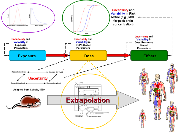
Uncertainty and Variability Sources in a cumulative risk assessment. Adapted from CompTox's Determining Uncertainty webpage.
Capabilities for Uncertainty Analysis
In the EPA's Office of Research and Development, the Ecosystems Research Division's Supercomputer for Model Uncertainty and Sensitivity Evaluation (SuperMUSE) is a key to enhancing quality assurance in environmental models and applications.
A fundamental characteristic of uncertainty and sensitivity analyses is their need for high levels of computational capacity to perform many relatively similar computer simulations, where only model inputs change during each simulation (Babendreier and Castleton, 2005).
SuperMUSE is computer network that enables researchers to conduct these computational intense sensitivity and uncertainty analyes.
Beneficial Aspects of SuperMUSE
- Scalable to individual user needs;
- Clustering from 2 to 2000+ PCs;
- Can handle PC models with 10's to 1000's of variables;
- Solves intensive computing problems (e.g. parametric sensitivity analysis);
- Simple and inexpensive;
- Ideal for debugging models (i.e., verification) and performing uncertainty and sensitivity analyses;
- With an average model runtime of 2 minutes, SuperMUSE can currently run over 4 million simulations/month.
Further Insight:
Babendreier, J. E. and K. J. Castleton. 2005. Investigating Uncertainty and Sensitivity in Integrated, Multimedia Environmental Models: Tools for FRAMES-3MRA. Environmental Modelling & Software. 20(8): 1043-1055.
![]()
Additional Web Resources:
- More information about SuperMUSE available from the Agency's Office of Research and Development
- The Multimedia, Multi-pathway, Multi-receptor Exposure and Risk Assessment (3MRA) technology
Summary: Uncertainty
Uncertainty is present and inherent throughout the modeling process and in this context is termed model uncertainty. Model uncertainty can arise from a lack of knowledge about natural processes, mathematical formulations and associated parameters, and/or data coverage and quality.
Model uncertainty is comprised of:
- Application niche uncertainty - uncertainty attributed to the appropriateness of a model for use under a specific set of conditions (i.e. a model application scenario). Also called 'scenario uncertainty'.
- Structure/framework uncertainty - incomplete knowledge about factors that control the behavior of the system being modeled; limitations in spatial or temporal resolution; and simplifications of the system.
- Parameter uncertainty - resulting from data measurement errors; inconsistencies between measured values and those used by the model.
“...uncertainty forces decision-makers to judge how probable it is that risks will be over-estimated or under-estimated for every member of the exposed population, whereas variability forces them to cope with the certainty that different individuals will be subjected to risks both above and below any reference point one chooses.” – NRC (1994)
“Models can never fully specify the systems that they described, and therefore are always subject to uncertainties that we cannot fully specify” – Oreskes (2003)
Summary: Sensitivity Analysis
Sensitivity analysis (SA) is the approach used to find the subset of inputs that are most responsible for variation in model output. A more rigorous analysis can relate the importance of uncertainty in inputs to uncertainty in model output(s) (EPA, 2003). Three levels of SA include:
- Screening - quick and simplistic, ranks input variables and ignores interactions between variables
- Local - works intensely around a specific set of input values (i.e., the local condition)
- Global - quantifies scale and shape of the input/output relationship; all input ranges; assesses parameter interaction
 for four models (HYDRUS, FECTUZ, CHAIN 2D, AND MULTIMED-DP).")
Sensitivity analysis of the van Genuchten parameter (a) for four models (HYDRUS, FECTUZ, CHAIN 2D, AND MULTIMED-DP). Image adapted from EPA (2002b).
Summary: Uncertainty Analysis
The end goal of an uncertainty analysis can be to characterize the uncertainty associated with the modeling results and identify the sources of this uncertainty. The uncertainty analysis should also meet the criteria determined at the onset of the modeling activity.
Often an uncertainty analysis is done to provide insight into areas of the project that could benefit from further research (e.g. parameter values, input data, model structure and underlying theory, etc.).
The idea of a tiered approach is to choose a level of detail and refinement for an uncertainty analysis that is appropriate to the assessment objective, data quality, information available, and importance of the decision (EPA, 2009b). An important feature of a tiered analysis is that the modeling and the accompanying uncertainty analysis may be refined in successive iterations (WHO, 2008)
Uncertainty analysis (UA) and sensitivity analysis (SA) are often carried out together so information about the sensitivity of the model to the variability of the inputs can be gained (EPA, 2009a).
A schematic of a tiered approach. Image adapted from EPA (2001b; 2004).
Further Insight into Sensitivity Analysis:
Literature and Guidance Documents:
- Guiding Principles for Monte Carlo Analysis. 1997. EPA-630-R-97-001. Risk Assessment Forum. U.S. Environmental Protection Agency. Washington, DC.
- Multimedia, Multipathway, and Multireceptor Risk Assessment (3MRA) Modeling System Volume IV: Evaluating Uncertainty and Sensitivity. 2003. EPA530-D-03-001d. Office of Research and Development. US Environmental Protection Agency. Athens, GA.
- Guidance on the Development, Evaluation, and Application of Environmental Models. 2009. EPA/100/K-09/003. Washington, DC. Office of the Science Advisor, US Environmental Protection Agency.
- Using Probabilistic Methods to Enhance the Role of Risk Analysis in Decision-Making With Case Study Examples DRAFT 2009 (PDF)(92 pp, 712 K, About PDF). EPA/100/R-09/001. Risk Assessment Forum. US Environmental Protection Agency. Washington, DC.
- Uncertainty and Variability in Physiologically Based Pharmacokinetic Models: Key Issues and Case Studies (PDF) (10 pp, 69 K, About PDF) 2008. EPA/600/R-08/090 Office of Research and Development. US Environmental Protection Agency. Washington, DC.
- Cullen, A. C. and H. C. Frey 1999. Probabilistic Techniques in Exposure Assessment: A Handbook for Dealing with Variability and Uncertainty in Models and Inputs. New York. Plenum Press.
- Frey, C. and S. Patil. 2002. Identification and Review of Sensitivity Analysis Methods. Risk Analysis 22(3): 553-578.
- Saltelli, A., K. Chan, and M. Scott, eds. 2000. Sensitivity Analysis. New York: John Wiley and Sons.
Agency Websites:
You Have Reached the End of the Sensitivity and Uncertainty Training Module

From here you can:
- Continue exploring this module by navigating the tabs and sub tabs
- Return to Training Module Homepage
- Continue on to another module:
- You can also access the Guidance Document on the Development, Evaluation and Application of Environmental Models, March, 2009.
References
- Addiscott, T. M. 1993. Simulation modelling and soil behaviour. Geoderma 60(1-4): 15-40.
- Beck, B., L. Mulkey and T. Barnwell. 1994. Model Validation for Exposure Assessments. DRAFT. Athens, GA: US Environmental Protection Agency.
- Babendreier, J. E. and K. J. Castleton. 2005. Investigating uncertainty and sensitivity in integrated, multimedia environmental models: tools for FRAMES-3MRA. Environ. Model. Software 20(8): 1043-1055.
- Cullen, A. C. and H. C. Frey 1999. Probabilistic Techniques in Exposure Assessment: A Handbook for Dealing with Variability and Uncertainty in Models and Inputs. New York. Plenum Press
- DOE (US Department of Energy). 2004. Concepts of Model Verification and Validation. LA-14167-MS. Los Alamos, NM. Los Alamos National Laboratory.
- EPA (US Environmental Protection Agency). 1995. Technical Guidance Manual for Developing Total Maximum Daily Loads. Book II: Streams and Rivers Part 1: Biochemical Oxygen Demand/Dissolved Oxygen and Nutrients/Eutrophication. EPA-823-B-95-007. Washington, DC. Office of Water.
- EPA (U.S. Environmental Protection Agency). 1997. Guiding Principles for Monte Carlo Analysis. EPA-630-R-97-001. Washington, DC. Risk Assessment Forum.
- EPA (US Environmental Protection Agency). 2001a. Probabilistic Aquatic Exposure Assessment for Pesticides I: Foundation (PDF).(49 pp, 1.3 MB, About PDF) EPA/600/R01/071. Research Triangle Park, NC. Office of Research and Development.
- EPA (US Environmental Protection Agency). 2001b. Risk Assessment Guidance for Superfund: Volume III - Part A, Process for Conducting Probabilistic Risk Assessment (PDF).(385 pp, 7.9 MB, About PDF) EPA 540-R-02-002. Washington, DC. Office of Emergency and Remedial Response.
- EPA (U.S. Environmental Protection Agency). 2002a. Guidance on Environmental Data Verification and Data Validation EPA QA/G-8 (PDF).(96 pp, 385 K, About PDF) EPA/240/R-02/004. Washington, DC. Office of Environmental Information.
- EPA (U.S. Environmental Protection Agency). 2002b. Simulating Radionuclide Fate and Transport in the Unsaturated Zone: Evaluation and Sensitivity Analyses of Select Computer Models. EPA/600/R-02/082. Cincinnati, OH. Office of Research and Development.
- EPA (US Environmental Protection Agency). 2003. Multimedia, Multipathway, and Multireceptor Risk Assessment (3MRA) Modeling System Volume IV: Evaluating Uncertainty and Sensitivity (PDF)(19 pp, 202 K, About PDF). EPA530-D-03-001d. Athens, GA. Office of Research and Development.
References (Continued)
- EPA (U.S. Environmental Protection Agency). 2004. Air Toxics Risk Assessment Reference Library Volume 1: Technical Resource Manual. EPA-453-K-04-001A. Research Triangle Park, NC. Office of Air Quality Planning and Standards.
- EPA (US Environmental Protection Agency). 2005. Excerpt from Baseline Ecological Risk Assessment for the International Smelting & Refining Site, Tooele County, Utah.
- EPA (US Environmental Protection Agency). 2006. Approaches for the Application of Physiologically Based Pharmacokinetic (PBPK) Models and Supporting Data in Risk Assessment. EPA/600/R-05/043F. Washington, DC. Office of Research and Development.
- EPA (US Environmental Protection Agency). 2009a. Guidance on the Development, Evaluation, and Application of Environmental Models. EPA/100/K-09/003. Washington, DC. Office of the Science Advisor.
- EPA (US Environmental Protection Agency). 2009b. Using Probabilistic Methods to Enhance the Role of Risk Analysis in Decision-Making With Case Study Examples. DRAFT. EPA/100/R-09/001 Washington, DC. Risk Assessment Forum.
- Frey, C. and S. Patil. 2002. Identification and Review of Sensitivity Analysis Methods. Risk Analysis 22(3): 553-578.
- Hanna, S. R. 1988. Air quality model evaluation and uncertainty. Journal of the Air Pollution Control Association 38(4): 406-412.
- Langstaff, J. E. (2007). Analysis of Uncertainty in Ozone Population Exposure Modeling. Technical Memorandum. Docket (OAR-2005-0172). Ambient Standards Group, Office of Air Quality Planning and Standards, U.S. Environmental Protection Agency. Research Triangle Park, NC.
- Matott, L. S., J. E. Babendreier and S. T. Purucker 2009. Evaluating uncertainty in integrated environmental models: A review of concepts and tools. Water Resour. Res. 45: Article Number: W06421.
- Morgan, G. and M. Henrion. 1990. Uncertainty: A Guide to Dealing with Uncertainty in Quantitative Risk and Policy Analysis.Cambridge, U.K. Cambridge University Press.
- NRC (National Research Council). 1994. Science and Judgment in Risk Assessment. Washington, DC. National Academies Press.
- NRC (National Research Council) 2007. Models in Environmental Regulatory Decision Making. Washington, DC. National Academies Press.
- Oreskes, N., K. Shrader-Frechette and K. Belitz. 1994. Verification, Validation, and Confirmation of Numerical Models in the Earth Sciences. Science 263(5147): 641-646.
- Oreskes, N., 2003. The role of quantitative models in science. In The Role of Models in Ecosystem Science. Eds. Charles D. Canham, Jonathan J. Cole and William K. Laurenroth. Princeton University Press. Pages 13-31.
References (Continued)
- Pascual, P. 2005. Wresting Environmental Decisions From an Uncertain World. Environmental Law Reporter 35: 10539-10549.
- Saltelli, A., K. Chan, and M. Scott, eds. 2000. Sensitivity Analysis. New York: John Wiley and Sons.
- Walker, W. E., P. Harremoës, J. Rotmans, J. P. van der Sluijs, M. B. A. van Asselt, P. Janssen and M. P. Krayer von Krauss 2003. Defining Uncertainty: A Conceptual Basis for Uncertainty Management in Model-Based Decision Support. Integrated Assessment 4(1): 5-17.
- WHO (World Health Organization). 2008. Uncertainty and Data Quality in Exposure Assessment Part 1: Guidance Document on Characterizing and Communicating Uncertainty in Exposure Assessment Part 2: Hallmarks of Data Quality in Chemical Exposure Assessment (PDF). (175 pp, 1.5 MB, About PDF) Exit Geneva, Switzerland. International Programme on Chemical Safety.