T-REX Version 1.5 User's Guide for Calculating Pesticide Residues on Avian and Mammalian Food Items
User's Guide T-REX Version 1.5 (Terrestrial Residue EXposure model)
March 22, 2012
Environmental Fate and Effects Division
Office of Pesticide Programs
U.S. Environmental Protection Agency
Washington, D.C.
On this page
- Introduction
- Guidance on T-REX Inputs
- T-REX Calculations and Results
- Risk Description Points to Consider
Appendices
- Guidance on Determining a Foliar Dissipation Half-life Parameter Value
- (Link to-) Initial Pesticide Residues on Arthropods
| T-REX User's Guide and Spreadsheet tool |
Contributors | QA/QC Officer | QA/QC Testers | QA/QC Reviewers |
|---|---|---|---|---|
|
|
|
|
|
The authors would also like to thank the members of the Terrestrial Biology and Terrestrial Exposure Technology Teams for their input and assistance in the development of this User's Guide and Spreadsheet.
-
Introduction
Welcome to the Terrestrial Residue EXposure (T-REX) model User's Guide. This document will provide directions on how to use T-REX and will explain how to estimate exposure concentrations and risk quotients for birds and mammals.
T-REX calculates the residues on avian and mammalian food items along with the dissipation rate of a chemical applied to foliar surfaces for single or multiple applications. Based on residue and dissipation rate calculations, this spreadsheet-based model also estimates acute and reproductive risk quotients. Using an adjusted LD50 method, T-REX calculates LD50 ft-2 values for both broadcast and banded (granular and liquid) applications. The results are presented by weight class for various sized birds and mammals for each type of application. Avian and mammalian risk quotients are also calculated for seed treatment applications for various crops.
T-REX, similar to the models FATE and TERREEC, calculates terrestrial exposure concentration estimates on plant surfaces following pesticide application. However, T-REX performs a number of calculations that neither FATE nor TERREEC perform. For example, T-REX adjusts acute and chronic toxicity values based on the relative body weight of the animal being assessed compared with the animal used in the toxicity studies. T-REX also calculates risk quotients for granular applications and seed treatments.
T-REX v.1.5 has undergone a formal internal Quality Assurance (QA) review in the Environmental Fate and Effects Division (EFED). A Quality Assurance Project Plan was developed and then approved by the project team and the QA Manager. If errors were identified, they were addressed and/or corrected.
Once T-REX is opened, the "READ ME" worksheet is displayed. This worksheet contains the version information, new model updates, and a list of references. Across the bottom of the Excel® window are several worksheet tabs, indicating the various functions performed by T-REX.
Important: When saving the workbook, select "Excel Macro-enabled Workbook" in the file type options.
The User's Guide provides guidance to the assessor on inputs needed to run T-REX (Section 2), describes the calculations performed by T-REX and the results (Section 3), and provides guidance on characterizing the results in the risk description of an ecological risk assessment (Section 4). This manual is intended to provide general guidance on the use of T-REX and is not intended to serve as a comprehensive guide on EFED's terrestrial risk assessment policies and methods.
-
Submitting Comments on T-REX, Version 1.5
The EFED user can submit comments on T-REX in the Comment worksheet. To submit a comment, type your last name in Cell B3 and your comment in Cell B6. Exit out of cell B6, then click on the "submit comment" button. A comment will not be sent unless you exit out of cell B6. These comments will be used in creating future versions of the model; therefore, all users are strongly encouraged to submit comments. Users need access to the EFED share drive (G: drive) for this function to work. Users without access to the share drive should contact Brian Anderson or Edward Odenkirchen, the program authors.
T-REX is designed to be easy to use, yet maintain a level of flexibility needed for the multitude of chemicals and use patterns encountered by risk assessors. T-REX may be used for foliar applications, seed treatments, or LD50/ft2 analysis. Specific guidance for each analysis is included in this User's Guide.
-
1.1 Summary of New Version Updates
T-REX version 1.5 replaces T-REX version 1.4.1. A summary of the updates/changes that were made to v.1.4.1 are listed below. This list of updates can also be found on the "Read Me" page of the T-REX v.1.5 model spreadsheet.
-
The T-REX User's Guide contains additional guidance regarding the foliar dissipation half-life input (Appendix A);
-
The estimates for pesticide concentrations on arthropod dietary items use empirical insect residue data from open literature and registrant-submitted studies (Appendix B);
-
An expanded list of seeding rates provided by the Biological and Economic Analysis Division is included for evaluating seed treatment exposure (Becker and Ratnayake, 2011);
-
Risk quotients are calculated for small, medium and large body weight classes for birds and mammals in seed treatment tab; and
-
The user can now designate variable application rates and interval spacing in inputs tab.
-
-
-
Guidance on T-REX Inputs
This section of the document provides guidance for entering parameters into T-REX to calculate risk indices for use in ecological risk assessments. Inputs include application data used to calculate estimated environmental concentrations (Section 2.1) and toxicity values (Section 2.2). Section 3 of this document describes how these input parameters are used by T-REX to calculate EECs and risk indices (risk quotients or LD50/ft2 values).
When T-REX is opened, a warning message may state "Security warning Macros have been disabled." In this case, click on options button to the right of the security warning, and select "Enable this content".
-
2.1. Entering Pesticide Application Data
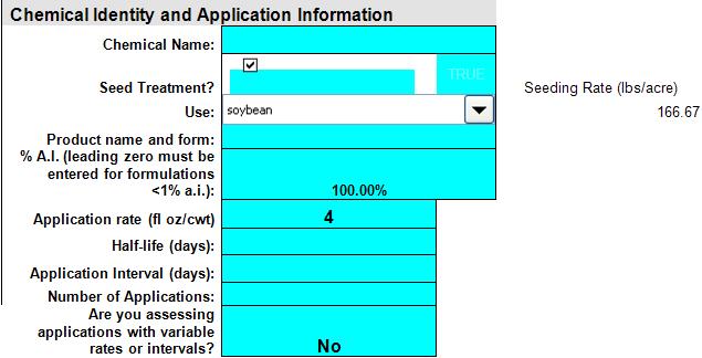
An "Inputs" worksheet (Figure 2-1) is included to increase consistency and transparency in the terrestrial exposure estimation process. With the exception of the seed treatment exposure and granular characterization worksheets, all necessary inputs may only be entered into the "Input" worksheet. Additional inputs needed for the seed treatment and granular characterization applications are described in Sections 2.4 and 3.2, respectively. A blue background designates an input cell (cells B6 ‐ B15, C41 ‐ C44, C50 ‐ C53, D48, D61, D65, E48, and E50 ‐ E53).
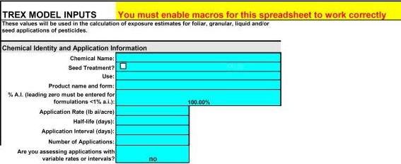 Figure 2-1
Inputs Screen in T-REX Version 1.5Inputs needed to run T-REX include the following (inputs denoted with an * are required; inputs denoted with an *a are required when multiple applications are being modeled:
T-REX Inputs Input Name Input Description Chemical name Enter either the chemical or common name used in the assessment. Seed treatment? Click on the box if you are assessing a seed treatment. If not, you do not need to select anything in this cell. Use Enter the type of use (e.g., turf, residential, crop, foliar, right-of-way, etc.) If applicable, also provide crop name. Product name and form Enter the name of the formulated product as it appears on the subject label, including any indication of the form of the product (e.g., 10g — 10% granular, wp — wettable powder, etc.) % A.I.* If an application rate for a formulated product is used, enter the % a.i. for the formulation. However, if the application rate has already been adjusted for % a.i., use 100%.
If the percent a.i. is < 1%, then a leading zero to the left of the decimal must be entered to ensure that 0.5% is not changed to 50% by EXCEL®. For example, a 0.5% formulation must be entered as "0.5" or ".5%" not ".5", and a 0.006% formulation must be entered as "0.006" or ".006%" not ".006".
Application Rate* Enter the maximum label application rate (pounds a.i./acre). If your application rate has already been adjusted for active ingredient, make sure you have entered 100 in the % a.i. cell above; otherwise, enter your application rate in lbs formulation/A here and then the % a.i. in the product in the above cell. Foliar Dissipation Half-life* Enter the foliar dissipation half-life in days. See Appendix A for guidance on determining the appropriate value for this parameter. The default chemical half-life is 35 days. Application Interval*a Enter the minimum interval (days) between multiple applications (if any). Note: This version of the model can only accommodate uniform application intervals; subsequent models may incorporate a provision of intervals of varying length. The risk assessor may evaluate the effect of using application intervals other than the minimum interval on the label to explore the effects of possible mitigation options on risk outcomes. Number of Applications*a Enter the number of applications. EFED policy states that screening-risk assessments should consider the maximum number of applications specified on the product label. However, the risk assessor may elect other numbers of applications to explore the effects of possible mitigation efforts on risk outcomes. Are you assessing applications with variable rates or intervals?*a Enter "yes" or "no". If "yes" is selected, you will enter the rate and intervals in Cells F6-35 and G6-35. You will not need to enter an application rate, interval or number of applications in Cells B11, B13 or B14. If "no" is selected, enter an application rate, interval and number of applications in Cells B11, B13 or B14. NOTE: "Clicking" the "reset model" button to the right of the first set of inputs will clear ALL of the user-supplied information. This button was included to allow the user to run multiple scenarios more quickly with T-REX without having to manually clear each cell.
-
2.2. Entering Toxicity Endpoint Data
To calculate risk quotients, user-supplied avian and mammalian toxicity endpoints need to be entered into the "Endpoints" section of the Inputs worksheet. These endpoints can be found in avian acute oral LD50, avian acute dietary LC50, avian reproduction NOAEC/L, acute mammalian LD50 or LC50, and mammalian reproduction NOAEC/L toxicity studies.
T-REX requires that both the chosen endpoint (entered in the blue cells C41 ‐ C44) and the test species be included (chosen from the drop-down menu options). For example, the user can enter an avian LD50 of 500 mg/kg-bw and this endpoint is based on a bobwhite quail study (i.e., chosen from the drop-down menu immediately to the right of the LD50 input cell). Typically, endpoint data for bobwhite quail, mallard duck, and laboratory rats from submitted studies or open literature will be used. In the case where data on bird species other than bobwhite quail or mallard duck are assessed (e.g., Japanese quail), the user should choose "other" from the species drop-down menu and enter the body weight of the species. A similar option for mammals is not currently available in this version of T-REX. Calculations for animals other than rats should be conducted by hand using equations included in this User's Guide.
-
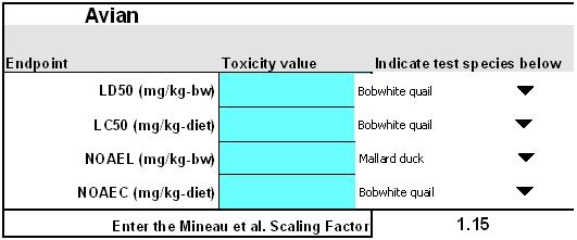
2.2.1. Avian Endpoints
The following avian toxicity endpoints may be entered into T-REX (Figure 2-2):
Avian Toxicity Endpoint Inputs Endpoint Name Avian Toxicity Endpoint Description LD50 Enter LD50 for dose-based acute effects endpoint (mg/kg-bw). LC50 Enter LC50 for dietary-based acute effects endpoint (mg/kg-diet). Reported Chronic Endpoint Enter NOAEL if reported in mg/kg-bw or NOAEC if reported in mg/kg-diet. Mineau Scaling Factor If chemical-specific data are available, the user can specify the avian scaling factor (see Mineau, et al.,1996) Otherwise, enter the EFED default value of (1.15). T-REX will not run unless a scaling factor is entered. However, a value of 1.0 can be entered if the assessor believes that body weight does not influence toxicity of the chemical being assessed. 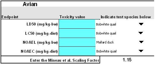 Figure 2-2
Avian Endpoints T-REX Version 1.5EFED policy states that for screening-level risk assessments, the lowest LD50, LC50, No-Observable-Adverse-Effect-Concentration (NOAEC) and/or No-Observable-Adverse-Effect-Level (NOAEL) from acceptable or supplemental studies should be used. For non-screening level risk assessments, the risk assessor may elect other values as necessary, but must document in the risk assessment why the lowest tested endpoint was not used. However, the assessor should determine that the lowest toxicity value from a laboratory study results in the lowest adjusted toxicity values for the various weight classes being assessed (See Section 3.1 for details on adjusted toxicity values). When toxicity values from different species are similar, it is important to indicate this similarity since T-REX adjusts the toxicity values based on body weight and food intake of the tested organism compared with the assessed organism. Thus, when data are available from multiple species, adjusted LD50s (described in Section 3) should be calculated for all species, and the lowest value should be used.
The risk assessor should note that this version of the model assumes a set body weight for tested bobwhite quail (178 g) and mallard duck (1580 g) unless another body weight is entered to the right of this cell or "other" is selected for a test species. Use of "other" species or studies involving subject animals markedly different from the assumed body weights requires the risk assessor to provide the alternate body weight and the species name. These data should be obtained from the study report if possible (time-weighted average). Alternatively, referenced body weight values may be obtained from a variety of sources, including USEPA (1993) and the testing laboratory.
-
2.2.2. Mammalian Endpoints
The following mammalian endpoints may be entered into T-REX (Figure 2-3):
Mammalian Toxicity Endpoint Inputs Endpoint Name Mammalian Toxicity Endpoint Description LD50 Enter LD50 (mg/kg-bw) for dose-based acute effects endpoint. LC50 Enter LC50 (mg/kg-diet) for dietary-based acute effects endpoint. Reported Chronic Endpoint Enter NOAEL if reported in mg/kg-bw or NOAEC if reported in mg/kg-diet.
Enter a NOAEL and/or NOAEC. To the right of the cell is a drop-down menu for the units in which the endpoint is expressed. The user may enter both a dietary concentration (NOAEC) and a daily dose (mg/kg-bw) if both are available. However, if both values are not available, then input "no" where T-REX asks if you have a dietary concentration or daily dose (T-REX will ask if you have the value not entered in Cell C30). If a dietary concentration and a daily dose are not both available, then the model will automatically make default adjustments for units to express the endpoint BOTH as NOAEC and NOAEL. The model will assume that a laboratory rat consumes 5% of its body weight daily (i.e., divide the concentration in food (ppm) by 20 to calculate the dose in mg/kg-bw). However, if a reproduction study reports toxicity values in units of dose (mg/kg-bw) and dietary concentration (mg/kg-diet), then both of these values should be used over the estimated values calculated by T-REX.
If a rat reproduction study is unavailable, the risk assessor may use the rat teratogenicity study NOAEL or NOAEC. In this case, the alternative endpoint should be identified and its limitations should be discussed in the risk description. Studies other than reproduction or developmental toxicity studies are not typically used by EFED to calculate risk quotients.
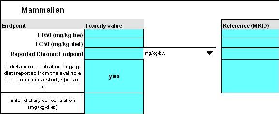 Figure 2-3
Mammalian Toxicity Endpoints T-REX Version 1.5The lowest LD50, LC50, NOAEC and/or NOAEL from acceptable or supplemental studies are used in screening-level risk assessments of mammals. For non-screening level assessments, the risk assessor may select other values as necessary, but must document in the risk assessment why the lowest tested endpoint was not used.
The risk assessor should note that this version of the model assumes a set body weight of 350 g for the tested organism, assuming they are laboratory rats. Use of other species or studies involving subject animals markedly different from the assumed body weight of 350 g will result in inaccuracies when extrapolating test endpoints to modeled animals. Thus, if a mammalian species other than a rat is used (e.g., dog, rabbit, and mink), the time-weighted average body weight of the animals that were tested in the experiment (from the DER or the original study report) should be used. Alternatively, reference body weight values may be obtained from a variety of sources including USEPA (1993) and the testing laboratory. However, T-REX does not currently allow the user to enter body weights of mammals that differ from the 350-gram laboratory rat. In this case, adjusted toxicity values would need to be performed by hand, using equations presented in this User's Guide.
-
-
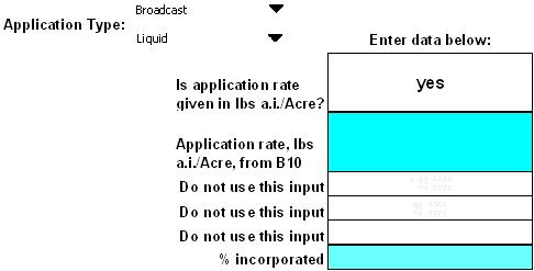
2.3. Additional Inputs for LD50 ft-2 Analysis
T-REX includes the capability to calculate the LD50 ft-2 risk index values with the user supplied information (Figure 2-4). Conceptually, an LD50 ft-2 is the amount of a pesticide estimated to kill 50% of exposed animals in each square foot of applied area. Although a square foot does not have defined ecological relevance, and any unit area could be used, risk presumably increases as the LD50/ft2 value increases. The LD50/ft2 value is used to estimate risk for granular formulations and row, banded, and in-furrow applications. For additional information on the LD50 ft-2 risk index, please refer to USEPA (1992). The LD50 ft-2 value is calculated using a toxicity value (adjusted LD50) and the EEC (mg a.i. ft-2) and is directly compared with the Agency's levels-of-concern (LOCs). Additional toxicity data are not needed for this calculation; however, additional information may be needed to allow for calculation of the exposure index (mg a.i./ft2). These data are described below.
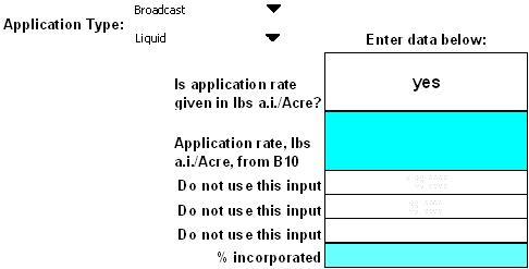 Figure 2-4
LD50 ft-2 inputsIn the first drop-down menu, choose the method of application from either "Broadcast" or "Rows/Band/In-furrow." The method of application is important in LD50 ft-2 calculations as it is linked to assumptions regarding the availability of the pesticide to wildlife. In the second drop-down menu, choose from either "Granular" or "Liquid." The application media is important for bioavailability assumptions for LD50 ft-2 calculations. Information regarding these inputs may be obtained from the product label.
Depending on the combination of application method chosen and characteristics of formulated product, the user will be prompted to enter the appropriate data in the blue cells located below and to the right of the drop-down menus (cells D61, D63 through D65). For broadcast applications of granular products, the user does not need to enter any additional information on the "inputs" page. However, if the product is a liquid applied as a broadcast spray or is a liquid or granular and is applied in rows, then additional information is needed. Guidance for entering data for each type of application is provided in Table 2-1 below. The user should pay attention to the units being requested for each input.
Table 2-1
Input Guidance for LD50 ft-2 AnalysisApplication Type Formulation Input Guidance Broadcast Granular % incorporated 0 % Liquid Fl oz. Product/Acre This value is either reported on the product label or can be calculated from the application rate reported in other units (e.g., lbs a.i./Acre) on the label. Rows/Band/In-furrow Granular or Liquid Row Spacing Row spacing is the amount of space (inches) between crop rows and is obtained from the product label. If data are not on the product label, the assessor may contact the Biological and Economic Analysis Division (BEAD) for typical values for the crop being assessed. Band width Band width is the width of the applied pesticide row (inches) and is obtained from the product label. If data are not on the product label, then the assessor may contact the Biological and Economic Analysis Division (BEAD) for typical values for the crop being assessed. % incorporated Value depends on the method of application:
- T-Banded — covered with specified amount of soil: 99%
- In-furrow, drill, or shanked-in: 99%
- Side-dress, banded, mix, or lightly incorporated with soil: 85%
- Broadcast, mix, or lightly incorporated: 85%
- Side-dress, banded, unincorporated: 0%
- Broadcast, aerial broadcast, unincorporated: 0%
Liquid Fl oz. Product/Acre This value is either reported on the product label or can be calculated from the application rate reported in other units (e.g., lbs a.i./Acre) Results are described in Section 3 of this document.
-
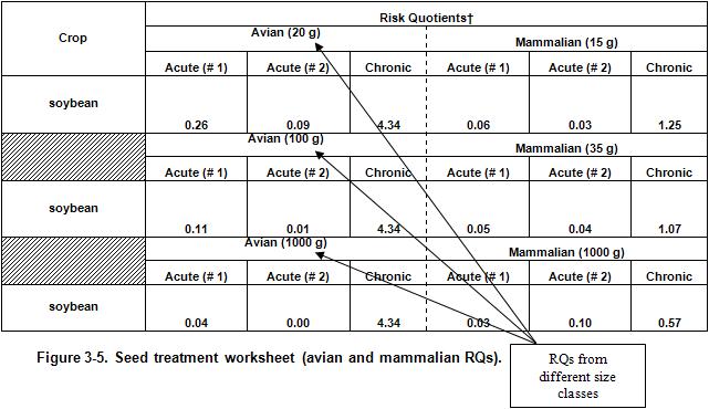
2.4. Additional Inputs for Seed Treatment Analysis
Because of the differences in foliar application and seed treatment uses of pesticides, the seed treatment worksheet (Figure 2-5) is used for estimating avian and mammalian Risk Quotients (RQs) for the various crops listed. Efforts were made to make the crop list as complete as possible with at least one crop from each crop group represented (from crop groups that could be seed treated). The Biological and Economic Analysis Division (BEAD) extensively reviewed seed treatable crops and associated seeding rates, which were provided to EFED, to create the most robust list of crops and rates possible. In this list, the most commonly seed treated crops (i.e., soybeans, corn, etc.) were listed first with fruiting and other vegetables listed further down the list in alphabetical order. This crop list also provides a complete list of references used by BEAD to compile the data.
If the assessment involves a seed treated crop, then the box labeled "Seed Treatment" on the "Inputs" tab should be checked, at which point a drop-down list of crops will appear. Once a crop is selected, the associated seeding rate will appear in the cell to the right of the drop-down box. After an application rate is entered, the "Seed Treatment" tab will provide all the intermediate calculations and RQs for use. The risk assessor can only run one crop at a time for seed treatments. Future versions of T-REX may allow multiple crops to be selected from the drop-down menu and allow simultaneous runs of the seed treatment analysis.
 Figure 2-5
Example of Inputs tab with seed treatment selectedThe chemical name, along with the reported and adjusted LD50 and NOAEC values for birds and mammals will automatically be carried over from the Inputs spreadsheet. Additional data input cells (in blue, cell location described below) that need to be entered are described below:
Additional Input Cells Requiring Data Entry Cell Name
(Location)Entry Description Product name and form
(Cell B9)Enter the product name for the seed treatment, as indicated on the label. Percent a.i. in formulation
(Cell B10)Enter the % active ingredient as a whole number (for example, 24% = 24) Application rate
(fl oz./cwt)
(Cell B11)These data are obtained from the product label. Only data on commodities being assessed need to be entered. For example, if rye is not an intended use, then it should be set to zero, as this will have no impact on the RQ calculations for the other crops. Density of product (lbs./gal)
(Cell J4)The density of the product is another input in the Seed Treatment tab (cell J4, orange background). This information can usually be found on the product label. If the density is unknown, the default value of 8.33 lbs/gallon will be used by the model (pre-entered in cell J4). NOTE: If a liquid rate is not available for a chemical, enter the dry weight application rate (lbs a.i./cwt) in the adjoining cell. Once this is done, however, the underlying equation in that cell has been replaced. It is preferable that users input the fl oz/cwt value.
-
-
T-REX Calculations and Results
This section of the User's Guide illustrates the T-REX output information that the user may incorporate into the assessment. The following figures are provided as an example only and the actual output will be dependent on the input parameters chosen from a specific usage pattern. The print area has been pre-set for each worksheet; therefore, "clicking" on the print button in the Excel® tool bar generates user-friendly outputs. Estimated Environmental Concentrations (EECs), adjusted toxicity values, and risk quotients (RQs) are calculated based on data entered in the input worksheet. These values, as applied to risk estimation from foliar sprays (dietary residue analysis), seed treatment applications, and LD50 ft-2 analysis, are presented below.
-
3.1. Risk Estimation Based on Dietary Residue Concentrations (Foliar Spray)
The methods used by T-REX to estimate risk from consumption of selected contaminated food items are described below. For this analysis, T-REX calculates EECs and risk quotients based on both the upper bound and mean residue concentrations for short grass, tall grass, broadleaf plants and fruits/seeds/pods as presented by Hoerger and Kenaga (1972) and modified by Fletcher et al. (1994). These concentrations are determined using nomograms that relate application rate of a pesticide to residues remaining on dietary items of terrestrial organisms. The results of the upper bound and mean residue levels are presented in separate tabs ("upper bound Kenaga" and "mean Kenaga"); however, the methods used to calculate EECs and risk quotients are equivalent. Concentrations on arthropod dietary items are based on available empirical residue data (Appendix B). Only RQs from the upper bound Kenaga worksheet should be used for comparison to levels of concern in the assessment. The mean residues and the RQs presented in the mean Kenaga worksheet are used only for risk description. Replacing the upper bound residues with the mean residues is not a valid mitigation approach when upper bound residues result in LOC exceedances. Based on the estimated dietary residue concentrations from the upper bound and mean Kenaga values, T-REX calculates the associated doses for various size classes of birds and mammals (Section 3.1.2). Both the dietary concentration (mg/kg-dietary item) and the resulting estimated doses (mg/kg-bw) may be used for risk estimation. The resulting dietary-based and concentration-based risk quotients are discussed in Section 3.1.4 of this User's Guide.
This section describes how T-REX estimates the following:
- residue concentrations on selected food items (mg/kg-dietary item)
- dose-based EECs (mg/kg-bw) from dietary concentrations on selected food items
- adjusted toxicity values
- risk quotients
-
3.1.1. Calculation of Dietary Concentrations on Selected Food Items
The spreadsheet calculates the pesticide residue concentrations on each selected food item on a daily interval for one year. When multiple applications are modeled, residue concentrations resulting from the final application and remaining residue from previous applications are summed. The maximum concentration calculated (out of the 365 days) is returned as the EEC used to estimate potential risk to birds and mammals as described below. Dissipation of a chemical applied to foliar surfaces for single or multiple applications is calculated assuming a first-order decay rate from the following first-order rate equation:
Ct = C0e-kt
or in natural log form:
ln(Ct) = ln(C0) - kt
Where:
Ct = concentration, parts per million (ppm), at time T.
C0 = concentration (ppm), present initially (on day zero) on the surface of selected food items. C0 is calculated by multiplying the application rate, in pounds active ingredient per acre, by 240 for short grass, 110 for tall grass, and 135 for broad-leafed plants, 15 for fruits/pods and 94 for arthropods for upper bound residue levels. Mean residue levels are derived by multiplying the application rate by 85 for short grass, 36 for tall grass, and 45 for broad-leafed plants, 7 for fruits/pods/seeds and 65 for arthropods. Residue levels for plants are based on work by Hoerger and Kenaga (1972) as modified by Fletcher et al. (1994). Residue levels of arthropods are based on an analysis completed by EFED of data from the scientific literature and registrant submitted studies (see Appendix B). Additional applications are converted from pounds active ingredient per acre to ppm on the plant surface and the additional mass added to the mass of the chemical still present on the surfaces on the day of application.
k = Exponential rate constant = ln 2 ÷ foliar dissipation half-life. This value is in cell R16 of the upper bound and mean Kenaga worksheets of T-REX.
t = time, in days, since the start of the simulation. The initial application is on day 0. The simulation is designed to run for 365 days.
The dietary concentrations, estimated using the above methodology, may be used directly to calculate risk quotients, but may also be used to calculate dose-based EECs (mg/kg-bw) for various size classes of mammals and birds as described in Section 3.1.2 below.
-
3.1.2. Calculating EEC Equivalent Doses Based on Estimated Dietary Concentrations on Selected Avian and Mammalian Food Items
EECs (mg/kg-bw) for various size classes of mammals and birds may be calculated based on the dietary residue concentrations that are derived using the equations presented above. To allow for this type of analysis, the EECs and toxicity values are adjusted based on food intake and body weight differences so that they are comparable for a given weight class of animal. The size classes assessed are
- small (20-gram),
- medium (100-gram), and
- large (1000-gram) birds,
and
- small (15-gram),
- medium (35-gram), and
- large (1000-gram) mammals.
Equations used to calculate food intake (grams/day) and to adjust toxicity values for dose-based risk quotients are presented below.
T-REX calculates food intake based on dry weight and wet weight of food items. The dose-based assessment uses the wet weight food consumption values by assuming that dietary items are 80% water by weight. However, if dietary items of a species that is being assessed are known, then a refined dose-based EEC can be calculated using appropriate water fractions of the food items.
Calculating Food Intake for Different Size Classes of Birds and Mammals
Daily food intake (g/day) is assumed to correlate with body weight using the following empirically derived equation (USEPA, 1993):
-
Avian consumption
F = (0.648 * BW0.651) / (1-W)
where:
F = food intake in grams of fresh weight per day (g/day)
BW = body mass of animal (g)
W = mass fraction of water in the food (EFED value = 0.8 for herbivores and insectivores, 0.1 for granivores)
Based on this equation, a 20-gram bird would consume 22.8 grams of food daily (114% of its body weight), a 100-gram bird would consume 65 grams of food daily (65% of its body weight daily), and a 1000-gram bird would consume 290 grams of food daily (29% of its body weight). These data, together with the residue concentrations (mg/kg-food item) on selected food items calculated from the Kenaga nomogram, are used to estimate the dose (mg/kg-bw) of residue consumed by the three size classes of birds as discussed below. Using a small (20-gram) bird as an example, a dietary concentration of 100 mg/kg-diet (ppm) x 1.14 kg diet/kg bw (114%) would result in an equivalent dose-based EEC of 114 mg/kg-bw.
A similar relationship between body weight and food intake has been derived for mammals (USEPA 1993):
-
Mammalian food consumption (g/day)
F = (0.621 * BW0.564) / (1 - W)
where:
F = food intake in grams of fresh weight per day (g/day)
BW = body mass of animal (g)
W = mass fraction of water in the food (EFED value = 0.8 for herbivores and insectivores, 0.1 for granivores)
The scaling factors, which result in a percent body weight consumed, are presented in the following table for each weight class of mammal. These values are used in the same manner as birds in calculating dose-based EECs (mg/kg-bw). Note the difference in food intake of granivores compared with herbivores and insectivores. This difference reflects the difference in the assumed mass fraction of water in their diets.
Scaling Factors for Mammals Organism and body weight Food intake (g day-1)a Percent body weight consumed (day-1)a Herbivores / Insectivores Granivores Herbivores / Insectivores Granivores 15 g 14.3 3.2 95 21 35 g 23 5.1 66 15 1000 g 150 34 15 3 aThe first number in this column is specific to herbivores/insectivores. The second number is for granivores. These groups have markedly different consumption requirements.
-
3.1.3. Calculating Adjusted Toxicity Values
The dose-based EECs (mg/kg-bw) derived above are compared with LD50 or NOAEL (mg/kg-bw) values from acceptable or supplemental toxicity studies that are adjusted for the size of the tested animal compared with the size of the animal being assessed (e.g., 20-gram bird). These exposure values are presented as mass of pesticide consumed per kg body weight of the animal being assessed (mg/kg-bw). EECs and toxicity values are relative to the animal's body weight (mg residue/kg bw) since consumption of the same mass of pesticide residue results in a higher body burden in small animals compared with large animals. For birds, only acute values (LD50s) are adjusted; dose-based risk quotients are not calculated for the chronic risk estimation. Adjusted mammalian LD50s and reproduction NOAELs (mg/kg-bw) are used to calculate dose-based acute and chronic risk quotients for 15-, 35-, and 1000-gram mammals. The following equations are used for the adjustment calculation (USEPA 1993):
-
Adjusted avian LD50
Adj. LD50 = LD50 (AW / TW)(x-1)
where:
Adj. LD50 = adjusted LD50 (mg/kg-bw) calculated by the equation
LD50 = endpoint reported from bird study (mg/kg-bw)
TW = body weight of tested animal (178g bobwhite; 1580g mallard)
AW = body weight of assessed animal (avian: 20g, 100g, and 1000g)
x = Mineau scaling factor for birds; EFED default 1.15
-
Adjusted mammalian NOAELs and LD50s (note that the same equation is used to adjust the NOAEL)
Adj. NOAEL or LD50 = NOAEL or LD50 (TW / AW)(0.25)
where:
Adj. NOAEL or LD50 = adjusted NOAEL or LD50 (mg/kg-bw)
NOAEL or LD50 = endpoint reported from mammal study (mg/kg-bw)
TW = body weight of tested animal (350g rat)
AW = body weight of assessed animal (15g, 35g, 1000g)
-
-
3.1.4. Calculating Risk Quotients
Two types of risk quotients are calculated by T-REX based on the estimated dietary residue concentrations determined from the Kenaga nomogram:
-
dietary based RQs and
-
dose based RQs.
These RQs are not equivalent. Dietary risk quotients are calculated by directly comparing the concentration of an administered pesticide (or estimated to be administered) to experimental animals in the diet in a toxicity study to the concentration estimated on selected food items. These risk quotients do not account for the fact that small animals need to consume more food relative to their body weight than large animals or that differential amounts of food are consumed depending on the water content and nutritive value of the food. The dose-based risk quotients do account for these factors. The dose-based RQs incorporate the ingestion rate-adjusted exposure from the various food items for the different weight classes of birds and the weight class-scaled toxicity endpoints. Formulas presented in Table 3-1 are used to calculate dose-based and dietary-based risk quotients:
Table 3-1
Formulas used to calculate dose- and dietary-based risk quotientsDuration Dose or Dietary RQ Surrogate Organism Equation Acute Dose-based Birds and mammals Acute Daily Exposure (mg/kg-bw) / adjusted LD50 (mg/kg-bw) Dietary-based Birds Kenaga EEC (mg/kg-food item) / LC50 (mg/kg-diet) Chronic Dietary-based Birds and mammals EEC (mg/kg-food item) / NOAEC (mg/kg-diet) Dose-based Mammals only EEC (mg/kg-bw) / Adjusted NOAEL (mg/kg-bw) These risk quotients are compared to the Agency's LOCs to determine if risk is greater than the levels of concern.
-
-
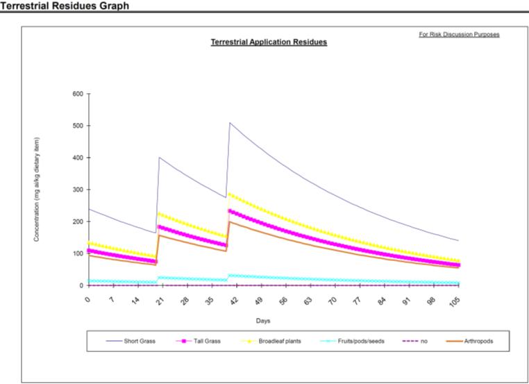
3.1.5. Graphs
The last section of the upper bound and mean Kenaga worksheets displays the terrestrial residues graph (Figure 3-1). The user can copy/paste this graph into a word processor document for use in the assessment. The accumulation and decline of the pesticide residues on each of the four food items are plotted over the first 100 days after the initial application. The "Graphs" worksheet provides similar graphs, but also includes mammalian and avian LOCs to allow the assessor to display the magnitude and duration of LOC exceedances in the assessment. These data are useful to include for risk discussion purposes.
 Figure 3-1
Kenaga residue worksheet (residue graph section)
-
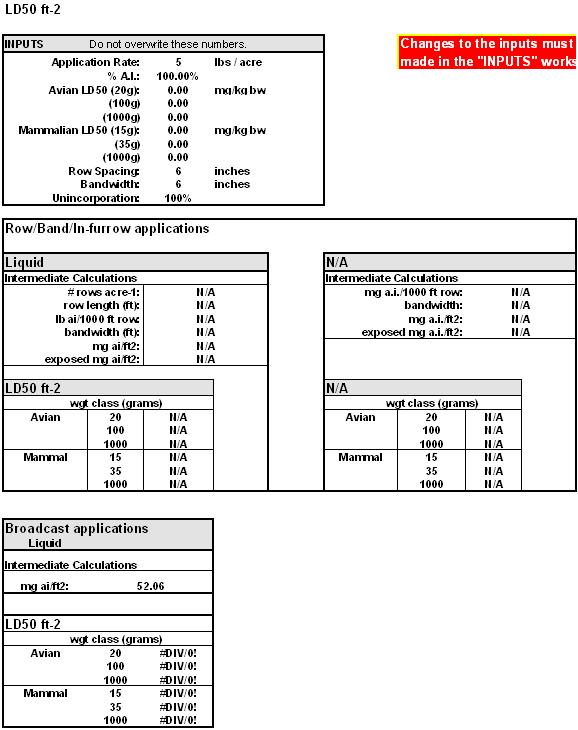
3.2. Results of LD50 ft-2 Analysis
Results of the LD50 ft-2 analysis are presented in the "LD50 ft-2" tab. Simply click on the LD50 ft-2 tab to display this page (Figure 3-2). There are three main sections in this worksheet:
- the input summary,
- row/band/in-furrow application summary, and
- broadcast application summary.
The input summary reiterates the parameters supplied by the user on the "input" worksheet. The other two sections calculate LD50 ft-2 values for row/band/in-furrow applications and broadcast applications, respectively. The calculations are based on a toxicity (adjusted LD50) and exposure (mg a.i./ft2) value. (Adjusted LD50s are discussed in Section 3.1.3). Equations used to calculate EECs are presented below for broadcast and banded granular and liquid applications. Percent incorporation in these equations for various application types entered by the assessor into T-REX is presented in Table 3-2.
Banded granular applications
mg a.i. ft-2 = (application rate in lbs a.i./A x % a.i. x 453,590 mg/lb) / (no. of rows A-1 x row length x bandwidth)
exposed mg a.i. ft-2 = mg a.i. ft-2 x % unincorporation
Banded liquid applications
mg a.i. ft-2 = (mg a.i. 1000 ft-1 row) / (1000 ft x bandwidth)
exposed mg a.i. ft-2 = mg a.i. ft-2 x % unincorporation
Broadcast granular applications
mg a.i. ft-2 = (application rate in lbs a.i./A x % a.i. x 453,590 mg/lb) / 43,560 ft2 acre-1
Broadcast liquid applications
mg a.i. ft-2 = (fl oz product A-1 x 28349 mg/oz x % a.i.) / 43,560 ft2 acre-1
Table 3-2
Percent incorporated assumed for several types of applications% incorporated - T-Banded covered with specified amount of soil: 99%
- in-furrow, drill, or shanked-in: 99%
- Side-dress, banded, mix, or lightly incorporate with soil: 85%
- Broadcast, mix, or lightly incorporated: 85%
- Side-dress, banded, surface application, unincorporated: 0%
- Broadcast, aerial broadcast, unincorporated: 0%
Based on these EECs, the LD50 ft-2 is calculated using the following equation:
LD50 ft-2 = EEC (mg a.i. ft-2) / (Adj LD50 ÷ bw (kg) of assessed animal)
The LD50/ft2 value is then compared with the Agency's levels of concern.
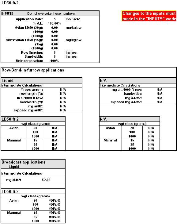 Figure 3-2
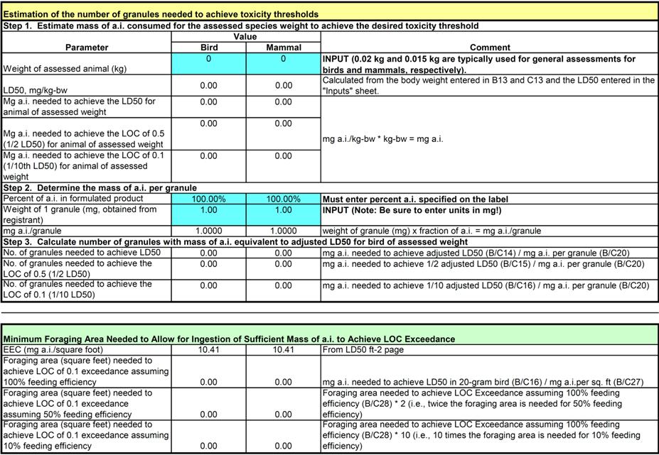
LD50 ft-2 worksheetThe worksheet "Granular Characterization Calcs" calculates the number of granules that need to be consumed by a bird to achieve a dose that would exceed the LD50 and trigger an LOC of 0.1 and an LOC of 0.5. There are four inputs (blue cells):
-
weight of an assessed bird (B14),
-
weight of assessed mammal (C14),
-
percent active ingredient in assessed product (B20 and C20) and
-
the weight of a single granule (B21 and C21).
Weight of an assessed bird is typically 20 grams (0.02 kg), but any weight may be entered. In addition, the minimum foraging area with sufficient number of granules to achieve a dose that exceeds the LD50 or 1/10th the LD50 is estimated by assuming that a bird consumes 100%, 50%, and 10% of the available granules.
 Figure 3-3
Granular Characterization Calcs Worksheet -
3.3. Results of Seed Treatment Applications
The seed treatment worksheet is organized into three main areas:
-
data input,
-
intermediate calculations, and
-
risk quotients.
The drop-down box on the Inputs tab of the model will allow the user to select a crop. When the application rates are entered, exposure and dose values are displayed in the intermediate calculations section (Figures 3-4 and 3-5). The application rates of the active ingredient (a.i.) and seeding rates are presented in the third and fourth columns, while the doses to birds and mammals and the exposed a.i. are displayed in the last three columns. The scaling factors used to adjust the reported LD50 values to all size classes of birds (20g , 100g, and 1000g) and all size classes of mammals (15g, 35g, and 1000 g) are also displayed for the risk assessor. The specific equations used for this adjustment were previously discussed in Section 3.1.3.
The seed treatment worksheet calculates the avian and mammalian dose (mg a.i. bw -1 day-1) and available pesticide (mg a.i. ft-2). Calculations of acute and chronic RQs for birds and mammals are described below.
Figure 3-4
Seed treatment worksheet (intermediate calculations section)Animal Size Crop Maximum
Application Rate
(lbs a.i./A)Maximum Seed
Application Rate
(mg a.i./kg seed)Avian
Nagy Dose
(mg a.i./kg-bw/day)Mammalian
Nagy Dose
(mg a.i./kg-bw/day)Available A.I.
(mg a.i. ft-2)Small soybean 0.22 1301.56 329.41 275.76 2.26 Medium 187.84 190.59 Large 84.10 44.19 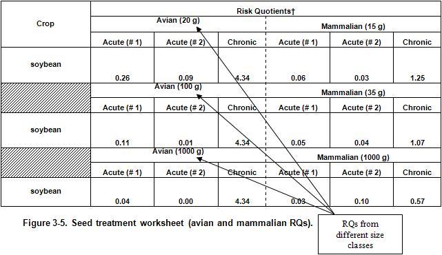 Figure 3-5
Seed treatment worksheet (avian and mammalian RQs)-
3.3.1. Calculation of Avian and Mammalian Doses (EECs)
As previously discussed, the following general equation is used to calculate doses from seed treatment applications using the scaling factor approach for a 20-gram bird and a 15-gram mammal:
Dose (mg/kg a.i. day-1) = (maximum seed application rate (mg a.i. kg seed-1) x scaling factor) / body weight of assessed animal.
Where:
Maximum Seed Application Rate (mg a.i./kg seed) = (Application rate x 10,000)
-
Application Rate (lbs a.i./cwt) = ( (Application rate (fl oz/cwt) x fraction of a.i. in formulation) / 128 fl oz/gallon) x density of product (lbs/gallon)
-
Maximum Application Rate (lbs a.i./A) = (Maximum seeding rate x application rate (lbs a.i./cwt)) / 100 lbs/cwt
Scaling factor
Equations presented in USEPA (1993) are used to adjust food intake and toxicity values to account for the differences in the size of the assessed animal compared with the size of the animal used in the toxicity tests. The doses used as the basis for risk quotient calculations are determined using the following equations and are referred to as Avian and Mammalian Nagy Doses in the seed treatment tab of T-REX:
Avian and Mammalian Nagy Dose (mg a.i./kg-bw) = (daily food intake g/day x 0.001 kg/g x maximum seed application rate (mg/kg-seed) / body weight of animal (kg)
Available a.i. (mg a.i./ft2) = The amount of available pesticide is calculated by converting the maximum application rate (lbs acre-1) to (mg a.i./ft2) using the following equation: (Maximum application rate (lbs/Acre) x 106 mg/kg) / (43,560 square feet/acre x 2.2 lb/kg)
-
-
3.3.2. Calculation of Risk Quotients for Seed Treatment Applications
Using the previously discussed methodology, RQs are calculated using the adjusted LD50 values for all weight classes of animals: 20g, 100g, and 1000 g for birds and 15g, 35g, and 1000 g for mammals. These calculations assume a tested body weight of 178 g for quail, 1580 g for duck, and 350 g for the lab rat. Acute RQs are calculated using two methods:
Method 1 (EEC/LD50 method)
Acute RQ = (mg a.i./kg bw/day) / adjusted LD50
Method 2 (analogous to the LD50 ft-2 method)
Acute RQ = (mg/kg a.i. ft-2) / (adjusted LD50 x body weight (kg))
These risk quotients are compared to the Agency's levels of concern for risk estimation. The appropriate risk quotient will be chemical specific although risk quotients derived from each method may be used to characterize risk.
Chronic RQs are calculated using the following equation:
Chronic RQ = mg a.i. kg-1 seed / NOAEC (mg/kg-diet).
Chronic RQs are adjusted to allow for an assessment of risk to different weight classes of mammals but not for birds as no data exist for incorporating scaling factors for birds.
-
-
3.4. Printing Results
The results from the upper bound Kenaga and LD50 ft-2 sheets are summarized in a separate worksheet titled "Print Results." This worksheet is designed so that the individual tables may be easily cut and pasted directly into Microsoft Word® documents with minimal formatting changes. This sheet is password protected; however, formatting changes (e.g., changing significant digits) are allowed. This worksheet includes all data that is included in the risk quotient calculations (EEC, Toxicity Value, and Risk Quotient).
-
-
Risk Description Points to Consider
-
4.1. Acute and Reproduction Dietary Discussions
The risk assessment includes numerous calculations of dietary exposure for multiple weight classes of animals. However, there are energetic considerations which suggest that some weight class/food item combinations are not likely to occur naturally. For example, there are not likely to be many 15 g mammals or 20 g birds that exclusively feed on vegetation. The risk assessor is urged to consult such texts as the Wildlife Exposure Factors Handbook (USEPA 1993), which will provide more comprehensive approaches for considering energy requirements and energy availability to estimate dietary exposure. In addition, the age of individuals may also play an important role in the types and relative amounts of food items selected. This factor should also be taken into account when describing dietary risks.
-
4.2. Acute Toxicity RQ Approaches
When effects data are available, dose-based and dietary-based acute RQs should be provided to risk managers. The dose-based approach assumes that the uptake and absorption kinetics of a gavage toxicity study approximate the absorption associated with uptake from a dietary matrix. Toxic response is a function of duration and intensity of exposure. Absorption kinetics across the gut and enzymatic activation/deactivation of a toxicant may be important and are likely variable across chemicals and species. For many compounds, a gavage dose represents a very short-term, high intensity exposure, whereas dietary exposure may involve a more prolonged exposure period. The dietary-based approach assumes that animals in the field are consuming food at a rate similar to that of confined laboratory animals. Energy content in food items differs between the field and the laboratory as do the energy requirements of wild and captive animals. The Wildlife Exposure Factors Handbook can provide insights into energy requirements of animals in the wild as well as energy content of their diets (USEPA, 1993).
-
4.3. Reproduction RQ Approach
The typical 21-week avian reproduction study does not define the true exposure duration needed to elicit the observed responses. The study protocol was designed to establish a steady-state tissue concentration for bioaccumulative compounds. For other pesticides, it is entirely possible that steady-state tissue concentrations are achieved earlier than the 21-week exposure period. Moreover, pesticides may exert effects at critical periods of the reproduction cycle; therefore, long-term exposure may not be necessary to elicit the effect observed in the 21-week protocol. The EFED screening-level risk assessment uses the single-day maximum estimated EEC as a conservative approach. The degree to which this exposure is conservative cannot be determined by the existing reproduction study. However, risk assessment discussions should be accompanied by the graphics from the T-REX model regarding the number of days dietary exposure is above the NOAEC. The greater number of days EECs exceed the NOAEC, the greater the confidence in predicting reproductive risk concerns.
-


References
Becker, Jonathan and Ratnayake, Sunil. 2011. Acres Planted per Day and Seeding Rates of Crops Grown in the United States. Biological and Economic Analysis Division (BEAD), Office of Pesticide Programs, United States Environmental Protection Agency.
Dunning, J.B. 1984. Body weights of 686 species of North American birds. Western Bird Banding Assoc. Monograph No. 1.
Fletcher, J.S., J.E. Nellesson and T. G. Pfleeger. 1994. Literature review and evaluation of the EPA food-chain (Kenaga) nomogram, an instrument for estimating pesticide residues on plants. Environ. Tox. And Chem. 13(9):1383-1391.
Hoerger, F. and E.E. Kenaga. 1972. Pesticide residues on plants: correlation of representative data as a basis for estimation of their magnitude in the environment. IN: F. Coulston and F. Corte, eds., Environmental Quality and Safety: Chemistry, Toxicology and Technology. Vol 1. George Theime Publishers, Stuttgart, Germany. pp. 9-28.
Mineau, P., B.T. Collins, A. Baril. 1996. On the use of scaling factors to improve interspecies extrapolation to acute toxicity in birds. Reg. Toxicol. Pharmacol. 24:24-29.
Urban, D. J. 2000. Guidance for conducting screening-level avian risk assessments for spray applications of pesticides. OPP/EFED, USEPA. July 7, 2000.
USEPA. 1992. Comparative analysis of acute avian risk from granular pesticides. Office of Pesticide Programs. USEPA. March 1992.
USEPA. 1993. Wildlife exposure factors handbook. Volume I of II. EPA/600/R-93/187a. Office of Research and Development, Washington, D.C. 20460.
USEPA. 1995. Great Lakes water quality technical support document for wildlife criteria. Office of Water, Washington D.C. Document Number EPA-820-B095-009.
Willis and McDowell. 1987. Pesticide persistence on foliage. Environ. Contam. Toxicol. 100:23-73.
T-REX Formulas (Version 1.5)
Converting NOAEC to/from NOAEL
If the reported chronic endpoint is mg/kg-diet (NOAEC) in a laboratory rat, then divide by 20 to get mg/kg-bw.
If the reported chronic endpoint is mg/kg-bw (NOAEL) in a laboratory rat, then multiply by 20 to get mg/kg-diet.
Adjusted LD50 (and also adjusted NOAEL for mammals)
The LD50 values entered on the input form are adjusted for animal class (20g, 100g and 1000 g birds and 15g, 35g, and 1000 g mammals), using the following equations: (The adjusted mammalian NOAEL uses the same equation as the adjusted mammal LD50).
- Avian LD50
Adj. LD50 = LD50 (AW / TW)(x-1)
- Mammal LD50
Adj. LD50 = LD50 (TW / AW)(0.25)
- Mammal NOAEL
Adj. NOAEL = NOAEL (TW / AW)(0.25)
where:
Adj. LD50 = adjusted LD50
LD50 = acute endpoint reported from bird or mammal study
TW = body weight of tested animal (178 g bobwhite; 1580 g mallard; 350 g rat)
AW = body weight of assessed animal (avian: 20 g, 100 g, 1000 g; mammals: 15 g, 35 g, 1000 g)
x = Mineau scaling factor for birds; EFED default 1.15
Scaling Factors
The following scaling factors (USEPA, 1993) are used in the consumption-weighted EECs:
- Avian consumption
F = (0.648 * BW0.651) / (1 - W)
- Mammal consumption
F = (0.621 * BW0.564) / (1 - W)
where:
F = food intake in grams of fresh weight per day
BW = body mass of animal (avian: 20 g, 100 g, 1000 g; mammal: 15 g, 35 g, 1000 g)
W = mass fraction of water in the food (0.8 for herbivores and insectivores, 0.1 for granivores)
Once the daily food intake values have been calculated using the scaling factors, the percent of the overall body weight represented by the daily food intake value for each weight class is calculated.
RQ Formulas Using Upper Bound Kenaga (EEC) Residues or Mean Kenaga Residues
EEC equivalent dose (mg/kg-bw) = upper bound EEC * (% body weight consumed/100)
Avian
Dose-based RQs = EEC equivalent dose / adjusted LD50
Dietary-based RQs
- Acute: EEC / LC50
- Chronic: EEC / NOAEC
Mammal
Dose-based RQs = EEC equivalent dose / adjusted N0AEL
Dietary-based RQs
- Acute: EEC / LC50
- Chronic: EEC / NOEAC
LD50 ft-2
Exposure Values
- Banded granular applications
mg a.i. ft-2 = (application rate x % a.i. x 453,590 mg/lb) / (no. of rows A-1 x row length x bandwidth)
exposed mg a.i. ft-2 = mg a.i. ft-2 x % unincorporation
- Banded liquid applications
mg a.i. ft-2 = (mg a.i. 1000 ft-1 row) / (1000 ft x bandwidth)
exposed mg a.i. ft-2 = mg a.i. ft-2 x % unincorporation
- Broadcast granular applications
mg a.i. ft-2 = (application rate x % a.i. x 453,590 mg/lb) / 43,560 ft2 acre-1
- Broadcast liquid applications
mg a.i. ft-2 = (fl oz product A-1 x 28349 mg/oz x % a.i.) / 43,560 ft2 acre-1
LD50 ft-2 Calculations
LD50 ft-2 (Avian) = (Exposed mg a.i. ft-2) / (Adjusted LD50 x .02)
LD50 ft-2 (Mammal)= (Exposed mg a.i. ft-2) / (Adjusted LD50 x .015)
Seed Treatments
The seed treatment worksheet calculates the avian and mammalian dose (mg a.i./kg-bw day-1), available pesticide (mg a.i. ft-2), and acute and chronic RQs for birds and mammals.
Adjusted LD50s are calculated as indicated previously. Only a 20 g bird and a 15 g mammal are assessed. The tested body weights are as follows: 178 g for quail, 1580 g for duck, and 350 g for the lab rat.
As discussed previously, doses are calculated using the scaling factor approach.
Maximum Seed Application Rate (mg a.i./kg seed) = (Application rate x 2.2 x 10⁶) / (100 x 2.2) = (Application rate x 10,000)
- Application Rate (lbs a.i./cwt) = (Application rate (fl oz/cwt) x decimal % of a.i. in formulation) / 128 fl oz/gallon) x density of product (lbs/gallon)
- Maximum Application Rate (lbs a.i./A) = (Maximum seeding rate x application rate (lbs a.i./cwt)) / 100 lbs/cwt
Avian and Mammalian Nagy Dose (mg a.i./kg-bw) = (daily food intake g/day x 0.001 kg/g x maximum seed application rate (mg/kg-seed) / body weight of animal (kg)
Available a.i. (mg a.i./ft2) = The amount of available pesticide is calculated by converting the maximum application rate in lbs acre-1 to mg a.i./ft2, using the following equation:
(Maximum application rate (lbs/Acre) x 106 mg/kg) / (43,560 square feet/acre x 2.2 lb/kg)
Acute and Chronic RQs
-
Acute RQ #1 = (Avian or Mammal) Nagy Dose / (adjusted LD50)
-
Acute RQ #2 = Available a.i. / (Adjusted LD50* kg body weight)
-
Chronic RQ = Maximum Seed Application Rate / NOAEC
Granular Characterization Calculations
Calculations are presented in Column D of the "Granular Characterization Calcs" worksheet of T-REX 1.5.
Appendix A
Guidance on Determining a Foliar Dissipation Half-life Parameter Value
The foliar dissipation half-life value is representative of the overall fate and transport of a pesticide relevant to foliar surfaces. Therefore, this half-life represents the chemical's degradation (i.e., through photolysis, hydrolysis and metabolism) and transport from leaf surfaces (i.e., through volatilization and washoff).
Foliar Dissipation Half-life Selection
EFED's default foliar dissipation half-life is 35 days, which can be applied to all pesticides without chemical-specific foliar dissipation half-lives. In using T-REX, the default foliar dissipation half-life of 35 days should be used first as a screening method for all chemicals, unless chemical-specific foliar dissipation half-lives (at least three) are readily available and values are > 35 days. If the estimated environmental concentrations (EECs) generated by T-REX with the default foliar dissipation half-life result in risk quotients (RQs) that are sufficient to exceed any levels of concern (LOCs), then the risk assessor should gather chemical-specific foliar dissipation half-lives.
It should be noted that in T-REX, the foliar dissipation half-life does not affect EECs when only one application is simulated. Therefore, in order to run T-REX for uses with only one application, it is not necessary for the risk assessor to obtain data to generate a chemical-specific half-life. However, in cases where a single application results in risks to animals, and the risk manager is interested in understanding the duration of the risk (i.e., how many days after the application the RQs exceed the LOC), then the risk assessor should consider obtaining chemical-specific half-life data.
If no RQs exceed the LOCs and there are no data to suggest that the foliar dissipation half-life may be above 35 days, the risk assessor does not need to re-run T-REX. Figure A.1 provides a decision framework for when to collect chemical-specific foliar dissipation half-lives.
 Figure A.1
Decision framework for when to collect chemical-specific foliar dissipation half-lives
Data Sources
The risk assessor can utilize several different data sources in order to determine an appropriate foliar dissipation half-life for a pesticide, including: studies submitted by the registrant (these are reviewed by the Health Effects Division (HED)) and studies from the scientific literature. These studies are listed in Table A.1 and described below.
| Study | Relevant Chemicals |
|---|---|
| Magnitude of the residue study: crop field trials (Guideline # 860.1500)* |
All |
| Magnitude of the residue study: field rotational crops (Guideline # 860.1900)* |
All |
| Magnitude of the residue study: irrigated crops (Guideline # 860.1400)* |
All |
| Dislodgeable foliar residue half-life of a pesticide (Guideline # 875.2100)* |
Non-systemic, low partitioning to plants (e.g., Kow < 0.01) |
| Willis and McDowell 1987** | All |
| Other studies available in the scientific literature | All |
* The guidelines can be obtained from Test Guidelines for Pesticides and Toxic Substances.
** Available on the G drive at the following location: G:\Models\Terrestrial Exposure\TREX\Current Model (approved for Risk Assessments)\Reference Documents
Registrant-submitted Magnitude of the Residue Studies
The following registrant-submitted studies may be used to determine a foliar-dissipation half-life for all chemicals:
-
Magnitude of the residue study: crop field trials (Guideline # 860.1500)
-
Magnitude of the residue study: field rotational crops (Guideline # 860.1900)
-
Magnitude of the residue study: irrigated crops (Guideline # 860.1400)
The Environmental Fate and Effects Division (EFED) risk assessor should acquire Data Evaluation Records (DERs) from HED for available studies that are classified as acceptable or supplemental. DERs for magnitude of the residue studies are available on HED's Chem Docs database. Magnitude of the residue studies may be used to estimate a foliar dissipation half-life when the following criteria are met:
-
Pesticides are applied to plants and data are available from treated foliage, fruits, seeds or grains (these are considered major food items in T-REX);
-
The residue decline data include a zero time point measurement. This measurement validates the amount of pesticides applied to the field and allows the dissipation curve to be based on the initial pesticide residues applied to the field;
-
The data include a minimum of three time point measurements, including the zero time point, for calculating a regression analysis. The three time points selected must demonstrate some dissipation of the pesticide.
-
Methods are sensitive enough to report the concentrations for at least three time points above the limit of detection (LOD) or limit of quantitation (LOQ).
In reviewing available magnitude of the residue studies for derivation of foliar dissipation half-lives, EFED scientists should consider whether the conditions of the studies may have led to atypically low half-lives. For example, a foliar dissipation half-life may have been underestimated in cases where a large precipitation event occurred prior to dissipation of 50% of the pesticide. In another example, the study may be conducted in a region and/or time when and where the pesticide is not typically used (e.g., study conducted in California during the summer for a semi-volatile pesticide that is used in the Great Lakes region during the winter).
If it is necessary for the EFED risk assessor to calculate the foliar dissipation half-life from submitted data, this can be accomplished by plotting the raw data (time vs. natural log transformed concentration) and determining the first-order exponential rate constant (k). The half-life value can be calculated as follows: Ln(2)/k.
Registrant-submitted Dislodgeable Foliar Residue Studies
Although data are often available to determine the dislodgeable foliar residue half-life of a pesticide (e.g., Guideline # 875.2100), these data are not considered useful for all chemicals in determining a foliar dissipation half-life parameter value for T-REX. Dislodgeable foliar residues are defined as: the amount of chemical that remains on the surface of the leaf and can be transferred from the leaf surface to objects that come into contact with or proximity to the leaf surface. For chemicals that are likely to sorb to plants (i.e., those with high Kow values) or those that are systemic, the dislodgeable foliar residue half-life could potentially underestimate the total foliar dissipation half-life, thereby overestimating the dissipation. In this case, the half-life would not account for the mass of pesticide contained within the plant or the differences in dissipation of pesticide residues on surfaces of the plant vs. pesticide residues within the plant. On the other hand, these data may be considered useful for chemicals that are not systemic and are not expected to partition to a great extent into the plant surfaces (e.g., Kow = 0.01 = 1% of chemical mass partitioning to plant lipids). The appropriateness of the use of data from dislodgeable foliar residue studies should be determined on a chemical by chemical basis. If dislodgeable foliar residue data are considered appropriate for a chemical, the risk assessor should consider the necessary study criteria noted above for the magnitude of the residue studies. DERs for dislodgeable foliar residue studies are available on HED's Chem Docs database.
Willis and McDowell 1987
Another source for dissipation data for wildlife exposure modeling purposes is Willis and McDowell (1987), which is available on the G drive at the following location: G:\Models\Terrestrial Exposure\TREX\Current Model (approved for Risk Assessments)\Reference Documents. This source contains data relevant to foliar dissipation half-lives of total (denoted by "T") and dislodgeable (denoted by "D") residues. Only total residue half-life values should be considered relevant for all chemicals in deriving the foliar dissipation half-life parameter value used in T-REX. If the risk assessor has determined that the dislodgeable foliar residue half-lives are appropriate for the assessed chemical, then these half-lives may also be considered.
Use of Foliar Dissipation Half-lives
Once data are available for characterizing the foliar dissipation half-life of a chemical, the EFED risk assessor should determine the 90th percentile upper confidence limit of all available values considered adequate for calculating the T-REX parameter value. If less than three foliar dissipation half-lives are available, the default foliar dissipation half-life value should be used. The EFED default foliar dissipation half-life value for T-REX is 35 days, which represents the upper bound of the half-lives reported by Willis and McDowell (1987).
When using the default half-life value, the risk assessor is urged to evaluate the effect of alternative assumptions of the residue half-life on the outcome of the terrestrial wildlife risk assessment and include this evaluation in the discussion of risk assessment uncertainties. Available data not used in generating the foliar dissipation half-life value for T-REX (such as those from unused dislodgeable residue studies or in cases where only 1 or 2 foliar dissipation half-life values are available) may be used for characterization purposes in a risk assessment (i.e., in the risk description). In addition, data from registrant-submitted soil residue dissipation studies (Guideline #875.2200) and terrestrial field dissipation studies (Guideline# 835.6100) may also be used for characterization of foliar dissipation half-lives. The risk assessor should note that data discussed in this paragraph should not be used to generate RQ values, but the data can be used to characterize the uncertainty associated with the RQ values reported in the risk estimation section of the assessment.