Development and Use of the Index Reservoir in Drinking Water Exposure Assessments
- Appendix A. Developing New Index Reservoir Scenarios for Tier II Modeling
- Appendix B. Spray Drift Scenario for the Index Reservoir
-
Tables
- Table 1. Example Table for Reporting EDWCs in the Drinking Water Exposure Assessment
- Table A-1. EXAMS Geometry for Index Reservoir
- Table A-2. EXAMS Dispersive Transport Parameters between Benthic and Littoral Layers in the Index Reservoir
- Table A-3. EXAMS Sediment Properties for the Index Reservoir
- Table A-4. EXAMS External Environmental and Location Parameters for the Index Reservoir
- Table A-5. EXAMS Biological Characterization Parameters for the Index Reservoir
- Table A-6. EXAMS Water Quality Parameters for the Index Reservoir
- Table B-1. Stream to Watershed Area Ratios for Some Representative Watersheds
- Table B-2. Estimates of Adjusted Spray Drift to the Index Reservoir as a Fraction of the Application Rate in Mass per Unit Area
-
Figures
- Figure 1. Index Reservoir Conceptual Model
- Figure B-1. Index Reservoir
MEMORANDUM
September 14, 2010
SUBJECT: Guidance on Development and Use of the Index Reservoir in Drinking Water Exposure Assessments
FROM: /s/ Donald Brady, Director, Environmental Fate and Effects Division (7507P), Office of Pesticide Programs
TO: Environmental Fate and Effects Division (7507P), Office of Pesticide Programs
Attached is the April 15, 20 10 document titled "Development and Use of the Index Reservoir in Drinking Water Exposure Assessments." The Guidance in this document is effective September 13, 2010. Changes and general updates from prior guidance on this topic include the following:
-
A separate value was developed for estimating spray drift resulting from air blast applications.
-
Consistent with the most recent DRAFT Input Parameter Guidance (EFED, 2009), the values for the application efficiency (APPEFF) parameter in PRZM have been included.
-
A new value of 600 meters has been estimated for the hydraulic length (HL) parameter in PRZM, and a description of how the estimate was made is included in a footnote. This change, which was instituted in December 1999, provides a more representative estimation of the eroded sediment load from the watershed.
-
A new and simpler method for estimating the total runoff for use in estimating the flow into the reservoir replaces the previous method. This change was instituted in the spring of 2000.
-
Watershed areas and spray drift factors in the previous document were in error and have been corrected.
-
Additional editorial corrections and clarifications were made.
In general, any drinking water modeling that begins on or after the week of September 13, 2010 should be conducted using the guidance discussed in the "Development and Use of the Index Reservoir in Drinking Water Exposure Assessments" document dated April 15, 2010.
Development and Use of the Index Reservoir in Drinking Water Exposure Assessments
R. David Jones, Kevin Costello, Jim Hetrick, Jim Lin, Ron Parker, Nelson Thurman, Chuck Peck
Office of Pesticide Programs
Environmental Protection Agency
April 15, 2010
Acknowledgements
The Office of Pesticide Programs, Environmental Fate and Effects Division would like to recognize and thank the following scientists for contributing to this report: Jim Breithaupt, Jim Carleton, Laurence Libelo, Robert Matzner, William Effland, and Ian Kennedy.
Summary of Revisions
This document updates and supersedes Guidance for Use of the Index Reservoir in Drinking Water Exposure Assessments, dated November 16, 1999. It also reflects changes in procedures, error corrections, and editorial modifications to improve clarity and completeness.
The following procedural changes were incorporated in this version of the guidance:
-
A separate value was developed for estimating spray drift from spray blast applications. Documentation for how this value was developed is included in Appendix B. Previously, spray blast applications were treated similar to aerial applications. With the development of a spray blast application value in the spring of 2000, users will be able to estimate more specific exposure levels from this application method.
-
Consistent with the most recent DRAFT Input Parameter Guidance (EFED, 2009), the values for the application efficiency (APPEFF) parameter in PRZM have been included.
-
A new value of 600 meters has been estimated for the hydraulic length (HL) parameter in PRZM, and a description of how the estimate was made is included in a footnote. This change, which was instituted in December 1999, provides a more representative estimation of the eroded sediment load from the watershed.
-
A new and simpler method for estimating the total runoff for use in estimating the flow into the reservoir replaces the previous method in Appendix A. This change was instituted in the spring of 2000.
The following error corrections were made:
-
The watershed areas in Table B-1 were corrected and reduced by a factor of 100. The other values in Table B-1 are correct.
-
The spray drift values in the Index Reservoir Guidance were inadvertently multiplied by the area of the reservoir. These values have been corrected.
Additions and clarifications included the following:
-
Previous guidance for the drift parameters for granular applications indicated that the parameters "need not be changed;" clarifying text in the revised version indicates that values should be set to 0.
-
Appendix B has been rearranged and additional explanatory material has been included to improve the clarity of this section.
-
Purpose
The purpose of this document is to provide guidance on the development and use of the index reservoir scenario for use in estimating pesticide concentrations in drinking water derived from vulnerable surface water supplies. Between 1996, after the passage of the Food Quality Protection Act (FQPA), and 2000, the Agency used the "standard pond" as an interim scenario for drinking water exposure. In 2000, the Agency implemented the index reservoir scenario to represent a watershed capable of supporting a drinking water facility that is prone to high pesticide concentrations. With the use of the index reservoir scenario, the Office of Pesticide Programs was able to improve the quality and accuracy of its models for estimating pesticide concentrations in drinking water.
This document reflects certain procedural changes that have evolved since the original guidance document was implemented in 2000. The updated version also contains a few minor error corrections in the documentation of the index reservoir scenario as well as editorial modifications to improve clarity and completeness.
This guidance document assumes that the user has previous experience in running the surface water models FIRST, PRZM, and EXAMS, and as such does not provide complete guidance on using these models to estimate drinking water exposure. Additional guidance for these models can be found in FIRST User's Manual, Environmental Fate and Effects Division, August 2001; PRZM-3, A Model for Predicting Pesticide and Nitrogen Fate in the Crop Root and Unsaturated Soil Zones: User's Manual for Release 3.12.2 by Carousel et al., 2005; Exposure Analysis Modeling System (EXAMS II) User Manual and System Documentation by Lawrence Burns, 2004; and Guidance for Selecting Input Parameters in Modeling the Environmental Fate and Transport of Pesticides, Version II, Environmental Fate and Effects Division, October 2009. These documents are available on the Internet at Models for Pesticide Risk Assessment.
Instructions for using the index reservoir scenario are provided in Section 2 of this document, while assumptions and limitations for the index reservoir scenario are included in Section 3: Reporting Results.
-
Development and Use of Index Reservoir Scenario
The index reservoir scenario is used in model simulations to estimate drinking water exposure and is intended as a replacement of the "standard pond," which is used to estimate wildlife exposure in aquatic ecosystems. It is used in a similar manner to the standard pond; however, flow rates have been modified to reflect local weather conditions and the area of the field and hydraulic length parameters have been modified to reflect values representative of the index reservoir. The use of the index reservoir as a standard watershed for drinking water exposure assessment was presented to the FIFRA Science Advisory Panel (SAP) in July, 1998, An Index Reservoir for Use in Assessing Drinking Water Exposure, Part IV of Proposed Methods for Basin-scale Estimation of Pesticide Concentrations in Flowing Water and Reservoirs for Tolerance Reassessment (Jones, et al., 1998). After reviewing the index reservoir scenario, the SAP (1988) recommended that the Agency implement the proposed approach.
The index reservoir represents potential drinking water exposure from a specific area with specific cropping patterns, weather, soils, and other factors. In general, a drinking water reservoir is a natural or artificial lake used to store water for use as drinking water by a local community. Reservoirs are usually fed by a number of streams, both perennial and ephemeral, which in turn are fed by precipitation and runoff from the surrounding watershed, as well as from groundwater discharge (see Figure 1). Pesticides applied to land near reservoirs and the streams that feed reservoirs can enter these waterbodies through runoff, spray drift, and leaching to groundwater.
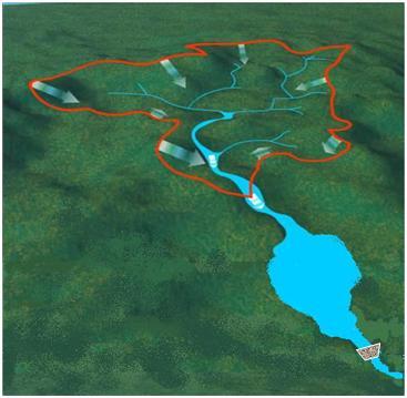 Figure 1. Index Reservoir Conceptual Model
The index reservoir scenario is used in Tier I and Tier II drinking water assessments. In a Tier I assessment, the FQPA Index Reservoir Screening Tool (FIRST) is used to develop estimated drinking water concentrations (EDWCs). If these values exceed the dietary risk, a Tier II analysis using PRZM/EXAMS is used.
Step 1. Determine Which Crops to Model
Identify the crop(s), maximum application rate(s), and appropriate application method(s) for each use specified on the label(s). In some cases, crops may be grouped together if they can be simulated using the same Tier I or Tier II model scenario. The appropriate crop location (in terms of the potential for runoff) and the application of the percent crop area (PCA) adjustment factor should also be identified. The reader should consult Development and Use of Percent Cropped Area Adjustment Factors in Drinking Water Exposure Assessments for a more detailed discussion on how to apply PCA adjustment factors.
Step 2. Setup and Run the Index Reservoir Models for the Crop(s) Being Simulated
The majority of the input parameters necessary to run the index reservoir scenario are similar for both the Tier I and Tier II drinking water assessments. The reader should consult Guidance for Selecting Input Parameters in Modeling the Environmental Fate and Transport of Pesticides for further information on these parameters. The following discussion provides additional guidance for conducting a Tier II assessment. If one of the PRZM/EXAMS shell programs such as PE or Express is not being used, or if the standard index reservoir scenario does not fit the pesticide application being considered, further guidance in Appendix A can be used to develop index reservoir scenarios and input files for PRZM and EXAMS.
The inputs for the index reservoir scenario have been standardized in the PRZM/EXAMS shell programs. The user should select the appropriate crop scenario and meteorological file, and select "ir298.exv" for the EXAMS Environment and "Reservoir" for the Field Size. The spray drift fraction should be set to reflect the spray drift loading for the PRZM/EXAMS transfer files. For aerial, orchard air blast, and ground spray applications, the assessor should use a value of 0.16, 0.063, and 0.064, respectively. An explanation for how these values were developed is in Appendix B. The application efficiency should be set to 0.95 for aerial and 0.99 for orchard air blast and ground spray applications. For granular applications and other applications methods that do not drift, the spray drift and application efficiency should be set to 0.00.
One of the last things to consider when running the index reservoir scenario is the PCA adjustment factor. The index reservoir scenario assumes that the entire area of the watershed is planted with the crop of interest (i.e., 100% crop coverage). For areas larger than a few hectares, such as most watersheds containing drinking water reservoirs, the entire area of the watershed is not planted with the crop of interest, so a PCA adjustment factor is employed. In FIRST, the user is prompted for a PCA adjustment factor during the model run, so the results are PCA-adjusted, i.e., adjusted by a factor that represents the maximum percent crop areas (as reported in the 1992 Agriculture Census) for the crop or crops under evaluation. In a Tier II assessment, however, the one-in-ten-year peak and average EDWCs developed using PRZM/EXAMs need to be post-processed in order to adjust them by the relevant PCA factor. The reader should consult the document Development and Use of Percent Crop Area Adjustment Factors in Drinking Water Exposure Assessments for a more detailed discussion on how to apply PCA adjustment factors.
-
Reporting Results
Tier I or Tier II results from simulations using the index reservoir should be included in drinking water exposure assessments, with the highest estimated exposure highlighted in the drinking water exposure assessment for use in OPP's dietary risk assessment. The one-in-ten-year peak value should be reported for use in assessing acute risk; the one-in-ten-year annual mean value should be reported for use in assessing chronic risk; and the 30-year mean value should be reported for use in assessing cancer risk. An example table, which can be used to summarize the EDWCs used for drinking water exposure assessment, is presented below (Table 1).
Table 1
Example Table for Reporting EDWCs Resulting in Drinking Water Exposure AssessmentCrop / Scenario 1-in-10 year annual peak concentration
(µg/L)1-in-10 year annual mean concentration
(µg/L)Overall Mean Concentration
(µg/L)Crop 1 Crop 2 Since 2005, OPP has been using the full distribution of drinking water exposure concentrations in combination with residues on food to develop probabilistic dietary exposure assessments. The distribution is used in a refined dietary assessment when the exposure estimates need to be refined.
When reporting results, it is important to include a discussion of the strengths and weaknesses of the index reservoir in the drinking water assessment. The following is standard language for describing the uncertainties in using the index reservoir for describing exposure to pesticides in surface water source drinking water. This language should be modified to suit the particular circumstances.
-
The index reservoir represents potential drinking water exposure from a specific area (Illinois) with specific cropping patterns, weather, soils, and other factors. Use of the index reservoir for areas with different climates, crops, pesticides used, sources of water (e.g., rivers instead of reservoirs), and hydrogeology creates uncertainties. In general, because the index reservoir represents a fairly vulnerable watershed, the exposure estimated with the index reservoir will likely be higher than the actual exposure for most drinking water sources. However, the index reservoir is not designed to represent a worst case scenario. Communities that derive their drinking water from smaller bodies of water with minimal outflow, or with more runoff prone soils, would be likely to have higher drinking water exposure than estimated using the index reservoir. Areas with a more humid climate that use a similar reservoir and cropping patterns may also have higher concentrations of pesticides in their drinking water than predicted using this scenario.
-
A single steady flow represents water flow through the reservoir. Because this steady discharge from the reservoir also removes chemicals, this assumption will underestimate removal from the reservoir during wet periods and will overestimate removal during dry periods. This assumption can both underestimate and overestimate the concentration of a pesticide remaining in the reservoir depending upon the annual precipitation pattern at the reservoir.
-
The index reservoir scenario uses the characteristics of a single soil to represent soils in the watershed. Soils can vary substantially across even small areas and this variability is not reflected in the scenario.
-
The index reservoir scenario does not consider tile drainage. Tile drainage contributes additional water and, in some cases, additional pesticide loading to the reservoir. This may cause either an increase or decrease in the pesticide concentration in the reservoir. Tile drainage also causes the surface soil to dry out faster, which will reduce runoff of the pesticide into the reservoir. The watershed used as the model for the index reservoir (Shipman City Lake) does not have tile drainage in the cropped areas.
-
The index reservoir scenario assumes complete mixing of the chemical through the water column. However, thermal stratification can occur in reservoirs that inhibits mixing. Eventually, an overturn event will occur that eliminates the stratification and returns the water column to a completely mixed state. Overturn occurs when the temperature drops in the fall and again in the spring when the reservoir warms up. EXAMS does not easily model stratification and spring and fall turnover. Because of this limitation with EXAMS, the Index Reservoir has been simulated without stratification. There are data to suggest that Shipman City Lake, upon which the Index Reservoir is based, does indeed stratify in the deepest parts of the lake at least in some years. This may result in both over and underestimation of the concentration in drinking water depending upon the time of the year and the depth of the drinking water intake.
-
-
Literature Cited
Burns, Lawrence A. 2004. Exposure Analysis Modeling System (EXAMS) User Manual and System Documentation. United States Environmental Protection Agency. Athens, Georgia. EPA/600/R-00/081, September, 2000, Revision G (May 2004).
Carousel, R.F., Imhoff, J.C., Hummel, P.R., Cheplick, J.M., Donigian Jr., A.S., Suárez, L.A. 2005. PRZM-3, A Model for Predicting Pesticide and Nitrogen Fate in the Crop Root and Unsaturated Soil Zones: Users Manual for Release 2.12.2.
Dunne, Thomas and Leopold, Luna B. 1978. Water in Environmental Planning. W. H. Freeman and Company, New York.
Environmental Fate and Effects Division. 2001. FIRST User's Manual. Office of Pesticide Programs, U. S. Environmental Protection Agency. August 1, 2001
Environmental Fate and Effects Division. 2009. Guidance for Selecting Input Parameters in Modeling the Environmental Fate and Transport of Pesticides, Version 2.1. Office of Pesticide Programs, U. S. Environmental Protection Agency. October 22, 2009
Jones, R. David, Abel, Sidney, Effland, William, Matzner, Robert, and Parker, Ronald. 1998. An Index Reservoir for Use in Assessing Drinking Water Exposure. Chapter IV in Proposed Methods for Basin-Scale Estimation of Pesticide Concentrations in Flowing Water and Reservoirs for Tolerance Reassessment., presented to the FIFRA Science Advisory Panel, July 29, 1998.
SAP. 1998. Federal Insecticide, Fungicide, And Rodenticide Act Scientific Advisory Panel Meeting: A Set of Scientific Issues Being Considered by the Agency in Connection with Proposed Methods for Basin-scale Estimation of Pesticide Concentrations in Flowing Water and Reservoirs for Tolerance Reassessment. FIFRA Scientific Advisory Panel Meeting, July 29, 1998, held at the Embassy Suites Hotel, Arlington, VA.
Teske, Milton E., Bird, Sandra L., Esterly, David M., Ray, Scott L., and Perry, Steven G. 1997. A User's Guide to AgDRIFT 1.0: A Tiered Approach for the Assessment of Spray Drift of Pesticides. Eight Draft. Spray Drift Task Force, Macon Georgia.
Appendix A
Developing New Index Reservoir Scenarios for Tier II Modeling
If the standard index reservoir scenario is not representative of the pesticide applications being assessed, the user will need to develop new PRZM and EXAMS input files. The following instructions should be used to develop new index reservoir scenarios. The instructions below are for PRZM and EXAMS and not the PRZM/EXAMS shell programs (i.e., PE and Express).
Step 1. Run PRZM to Obtain the Runoff Volume for the Watershed
The index reservoir scenario needs to take into account flow through the waterbody. The flow-rate parameter is estimated using PRZM and the weather file for the local weather station where the scenario is located. The estimated mean runoff from the watershed is used to estimate the volume of flow through the reservoir. Use of the mean runoff is justified on the basis that the duration of the runoff pulses, as well as the variation in daily flows, is small relative to the residence time in the reservoir, and that the reservoir has some hydrologic buffering.
Since EXAMS assumes that the volume of the waterbody is constant, the flow out of the reservoir must equal the flow into the reservoir. As such, the discharge rate from the reservoir is set equal to the influent flow rate. The STFLO (or STream FLOws) parameter is used to set the flow into the reservoir from upstream. The units on STFLO are m3/hr. STFLO can be set into each segment for each month during the year. All of the flow is set to enter the water column (segment 1). Currently all monthly flow values are set to the same value.
PRZM should be run with the scenario set for the index reservoir site that is to be simulated. It is not necessary to simulate pesticide applications during this run. The user should then modify record 45, which is the card for turning on and specifying the number and kind of optional outputs, and record 46, which specifies which optional outputs to produce. For record 45, set the NPLOTS variable to 1 for one output variable, and for record 46, set the PLNAME variable to RUNF and MODE to TCUM. Other variables in record 46 should be commented out by placing a "***" at the start of line. PRZM will place the cumulative daily runoff depth in centimeters in the times series output file. The name of this file is designated in the PRZM command file (.RUN), and usually is given a default "ZTS" extension. The units on the output are cm, not cm per day as indicated in the PRZM manual. As the estimate is cumulative, the last value in the file is the total runoff depth over the period of the simulation.
Step 2. Calculate the Mean Overall Stream Flow Rate
The total runoff depth should be divided by 100 to convert the result to meters. Multiply this number by the area of the index reservoir watershed in square meters (1,728,000 m2) to obtain the total volume of runoff from the watershed over the period of the simulation. Divide this number by the years in the simulation to get the mean annual runoff value. Then, divide by 8760 (365 d/yr * 24 h/d) to obtain the overall mean flow on an hourly basis, which are the units for the STFLO parameter in EXAMS.
Step 3. Set the STFLO Parameter for the Scenario in EXAMS
Start EXAMS and set the Mode variable equal to 3 (continuous mode). Then, read the Standard Index Reservoir, IndexRes.Exv, into EXAMS using the command: READ Env ir298.Exv. The parameter values used to derive the Standard Index Reservoir file are provided in Table A-1 through A-7. Note that EXAMS must be in the directory where the Exv file is located; otherwise, the directory location must be included with the filename. STFLO is an array variable with two dimensions. The first dimension is an index, which indicates the compartment the stream is flowing into, and the second index is the month of the year. The STFLO for compartment 1 (the water column) is set to the mean runoff flow, obtained in Step 2, for each month, and the STFLO for compartment 2 (the benthic layer) is set to 0. The commands for setting these values are:
Set STFLO(1,*) = nnn.n
Set STFLO(2,*) = 0
where nnn.n is the hourly runoff flow from Step 2. The "*" sets all cells for all months equal to that specified value.
Step 4. Rename the Scenario
First, set the EXAMS database name command to give the scenario a new name. This is the name that is shown when the scenario is in the EXAMS User Database (UDB) and appears when issuing the CATALOG command. Include the crop and location in the name. For example, an index reservoir name for use with almonds might be "Index reservoir for Kern Co, CA almonds." The command to set the name using this example is:
Env Name is Index reservoir for Kern Co, CA almonds
After setting the name, save the scenario to an external file using the WRITE command. For example:
WRITE env IRCAAlmd.Exv
It is recommended that the name start with "IR" to indicate that it is an index reservoir scenario and the extension be set to "EXV" for EXAMS environment file.
If the scenario is to be placed in the EXAMS user data base, use the STORE command:
STORE env nn
where nn is the number of the location in the database the scenario is to be stored. Make sure not to overwrite another scenario in the database when saving the scenario.
Step 5. Approval of the Scenario
After the scenario is constructed, it must be approved by the Water Quality Tech Team (WQTT). For the review process, the user should include the PRZM and EXAMS scenario files as well as a brief description and justification for the scenario. In those cases where the scenario description was written for use with the standard pond, the description can be modified to include information on the index reservoir. If the scenario description has not been developed, the description should include information on the soil and location. The location selected should represent a vulnerable site that can be used to produce the crop being modeled. Approval of new scenarios by the WQTT will be consistent with EFED's memorandum WQTT Advisory Note: The Environmental Fate and Effects Division's Internal Quality Assurance Review Process for Proposed PRZM Scenarios, dated May 9, 2007. Once a scenario becomes final, the WQTT tech team co-chair(s) will be responsible for updating the approved scenarios available on the Models for Pesticide Risk Assessment web site.
Step 6. Determine Which Crops to Model
Select the crop use or uses which are anticipated to result in the maximum loading of a pesticide into the surface waterbody via runoff. In some cases, PRZM and EXAMS simulations on more than one crop may be necessary in order to decide which crop produces the highest EDWCs and whether any back-calculated Drinking Water Levels of Comparison (DWLOC) may be exceeded. The selection of an appropriate crop or crops for modeling must consider the maximum application rate, location in terms of the potential for runoff, and the impact of applying the PCA adjustment factor on the EXAMS output. It should be noted that the PCA adjustment reduces the estimates of pesticide concentrations in drinking water and as such a use other than that associated with the maximum labeled application rate may result in a higher estimated pesticide concentration depending on the geographic limitations of the crops and the labeled uses. The reader should consult Development and Use of Percent Crop Area Adjustment Factors in Drinking Water Exposure Assessments for a more detailed discussion on how to apply PCA adjustment factors.
Step 7. Modify the Index Reservoir Input Files for the Crop Being Simulated
Using the PRZM input file developed in Step 1, modify the area of the field (AFIELD) and hydraulic length (HL) parameters. Set the AFIELD parameter, the fourth parameter on record 7 of the PRZM 3 input (.INP) file, to 172.8. This is the number of hectares in the index reservoir watershed. (This does not include the area of the reservoir itself). The seventh parameter in the same record is the hydraulic length (HL). This parameter is used to calculate the eroded sediment load from the watershed and should be set to 600 meters1. The DRFT parameter in record 16 of the PRZM input file needs to be set to reflect the spray drift loading for the PRZM-EXAMS transfer files. For aerial applications, use a value of 0.16. Use 0.063 for orchard air blast, and 0.064 for ground spray. An explanation for how these values were developed can be found in Appendix B. The APPEFF parameter should be set to 0.95 for aerial and 0.99 for orchard air blast and ground spray. The spray drift parameters should be set to 0.00 for granular applications.
1The value for the HL parameter was estimated by identifying the longest overland flow path from the edge of the watershed to an identifiable channel. This was done using the USGS 7.5 Minutes Series Map of the Shipman, Illinois Quadrangle, dated 1983. This distance is approximately 600 m.
Step 8. Establishing EXAMS Command File
The EXAMS command file, which usually has an ".EXA" extension, needs to be modified slightly so that EXAMS loads the index reservoir rather than the standard pond. (Note the difference in file extensions: EXAMS environment files often have "EXV" extensions.) If the EXAMS scenario is read from an external file, use the index reservoir environment file rather than the standard pond file. For example:
read env indexres.exv
If using the internal user database, use the load command followed by the position of the index reservoir in the database. If the index reservoir was saved in position 6 in Step 4 above then use:
recall env 6
in the EXAMS command file to load the index reservoir.
Once the file has been loaded into EXAMS, the procedure for running the index reservoir simulation is identical to that used in running simulations for the standard pond.
| Parameter | Littoral | Benthic | Source |
|---|---|---|---|
| Area (AREA) | 52,609 m2 | 52,609 m2 | Jones et al., 1998 |
| Depth (DEPTH) | 2.74 m | 0.05 m | Jones et al., 1998 |
| Volume (VOL) | 144,000 m3 | 2630 m3 | Jones et al., 1998 |
| Length (LENG) | 640 m | 640 m | estimated from map |
| Width (WIDTH) | 82.2 m | 82.2 m | estimated from map |
| Stream Flow (STFLO) | variable | 0 m3 h-1 | see text |
| Parameter | Path 1* | Source |
|---|---|---|
| Turbulent Cross-section (XSTUR) | 52609 m2 | Burns, 1997 |
| Characteristic Length (CHARL) | 1.395 m | Burns, 1997 |
| Dispersion Coefficient for Eddy Diffusivity (DSP)** | 3.0 x 10⁻⁵ | standard pond |
* JTURB(1) = 1, ITURB(1) = 2; ** each monthly parameter set to this value.
| Parameter | Littoral | Benthic | Source |
|---|---|---|---|
| Suspended Sediment (SUSED) | 30 mg L-1 | standard pond | |
| Bulk Density (BULKD) | 1.85 g cm-3 | standard pond | |
| Percent Water in Benthic Sediments (PCTWA) | 137% | standard pond | |
| Fraction of Organic Matter (FROC) | 0.04 | 0.04 | standard pond |
| Parameter | Value | Source |
|---|---|---|
| Precipitation (RAIN) | 0 mm month-1 | |
| Atmospheric Turbulence (ATURB) | 2.00 km | standard pond |
| Evaporation Rate (EVAP) | 0 mm month-1 | |
| Wind Speed (WIND) | 1 m sec-1 | standard pond |
| Air Mass Type (AIRTY) | Rural (R) | |
| Elevation (ELEV) | 54.9 m | USGS map |
| Latitude (LAT) | 39.12° N | USGS map |
| Longitude (LONG) | 90.05° W | USGS map |
1 Default values provided were used in development of index reservoir scenario. These values will be overwritten when the meteorological file is processed by EXAMS.
| Parameter | Limnic | Benthic | Source |
|---|---|---|---|
| Bacterial Plankton Population Density (BACPL) | 1 cfu cm-3 | see text | |
| Benthic Bacteria Population Density (BNBAC) | 37 cfu (100 g)-1 | see text | |
| Bacterial Plankton Biomass (PLMAS) | 0.40 mg L-1 | standard pond | |
| Benthic Bacteria Biomass (BNMAS) | 6.0x10⁻³ g m-2 | standard pond |
| Parameter | Value | Source |
|---|---|---|
| Optical path length distribution factor (DFAC) | 1.19 | standard pond |
| Dissolved organic carbon (DOC) | 5 mg L-1 | standard pond |
| chlorophylls and pheophytins (CHL) | 5x10⁻³ mg L-1 | standard pond |
| pH (PH) | 7 | standard pond |
| pOH (POH) | 7 | standard pond |
Appendix B
Spray Drift Scenario for the Index Reservoir
Spray drift can enter the reservoir both directly from fields alongside the reservoir and from drift into streams in the reservoir's watershed. In estimating spray drift for the index reservoir, OPP estimates the drift component for these two sections separately and then combines the estimates. This appendix describes the stream network and reservoir geometry, the general assumptions used to estimate the spray drift for the index reservoir, and the calculations of spray drift contributions to the streams and the reservoir.
-
Stream Network and Reservoir Geometry
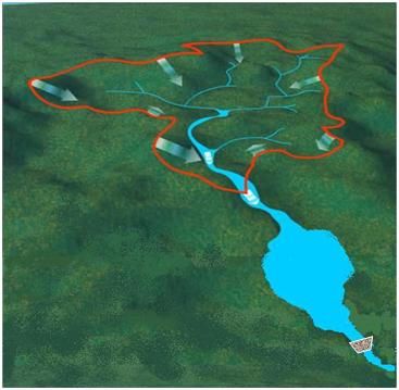
The spray drift scenario for the index reservoir is based on the geometric characteristics of the watershed and the reservoir. Spray drift can enter the reservoir both directly from fields along side the reservoir and from drift into streams in the reservoir's watershed. A schematic diagram for the index reservoir is provided in Figure B-1. The index reservoir is approximately 82 m wide and 640 m long, with an area of 5.3 ha (Jones et al., 1998). The area of the entire watershed is 172.8 ha.
 Figure B-1. Index Reservoir
-
General Assumptions Used to Estimate the Spray Drift for the Index Reservoir
As an initial assumption, the watershed is assumed to be 100% planted in the crop being modeled. This assumption was subsequently modified with application of a percent crop area (PCA) adjustment factor, which is applied to the final modeling estimates. Spray drift can enter the reservoir directly from application to fields alongside the reservoir and from the streams in the watershed of the reservoir that intercept spray drift. A small non-treated area, or buffer, of 4 meters is assumed to exist on either side of the streams in the watershed and represents the stream shoreline below the high water line. This assumption was based on the conditions observed in the watershed of the Shipman Reservoir, which was used to develop the index reservoir scenario. No buffers are assumed to exist in the ephemeral portion of the stream (e.g., the headwaters), as it is assumed that this area is plowed as a regular part of the field and receives a full pesticide application. In addition, no buffer is assumed to exist around the reservoir itself for two reasons. First, in some cases, crops are grown close to the edge of the waterbody. For example, apple orchards in the Columbia River basin are often planted in the bottomland along the river shore. Secondly, many pesticide labels do not have spray drift buffer requirements. This assumption may be adjusted if pesticide labels do restrict applications to a specific distance from waterbodies.
In order to estimate the portion of spray drift contributed by the stream network to the reservoir, an estimate of the length and width of the streams in the watershed is needed. These measurements were estimated based on the configuration of the index reservoir, designed based on the Shipman Reservoir in Shipman, Illinois. In order to estimate the stream length, the density of streams above Shipman City Lake was assumed to be similar to that for the Macoupin Creek drainage, which included the Shipman Watershed (and for which such data were available). Estimates of stream density for the Macoupin Creek watershed and several other drinking water system watersheds are presented in Table B-1. These estimates were made separately for perennial streams and for all (perennial + ephemeral) streams in the watershed. Perennial streams flow year round; ephemeral streams only flow periodically, for example, when there has been substantial precipitation in the basin. Based on the watersheds considered, the Macoupin Creek watershed contains the lowest density of perennial streams and the highest density of all streams in the watershed. Based on the density estimate for the Macoupin Creek watershed, and the area of the Shipman watershed, the index reservoir is assumed to have 550 meters of perennial streams and 950 meters of ephemeral streams, for a total of 1500 meters for all streams.
The mean width of the streams in the index reservoir was estimated using a nomogram (Dunne and Leopold, 1978). Estimates from the nomogram are available for several regions in the United States. The estimate used for the Index Reservoir spray drift scenario is representative of the eastern United States. Based on the drainage area of the Index Reservoir watershed, the mean stream width for all streams in the watershed is estimated to be 4 meters. As described above, a buffer of 4 meters has also been assumed for perennial streams, resulting in an area where crops cannot be planted and therefore will not be treated with pesticide. The assumed total area of the stream network in the index reservoir watershed consists of 2200 m2 of perennial streams and 3800 m2 of ephemeral streams, for a combined land area of 6000 m2.
Table B-1
Stream to Watershed Area Ratios for Some Representative Watersheds*Watershed Total Stream Length (m) Area (m2) Drainage Density (m/m2) Perennial All (perennial + ephemeral) Perennial All (perennial + ephemeral) Macoupin Creek**, IL 804,600 2,188,700 2,527,800,000 3.18 x 10⁻⁴ 8.66 x 10⁻⁴ Blue Marsh Reservoir, PA 2,478,400 3,089,900 4,946,900,000 5.01 x 10⁻⁴ 6.25 x 10⁻⁴ Occoquan Creek, VA 1,717,200 2,397,900 3,418,800,000 5.02 x 10⁻⁴ 7.01 x 10⁻⁴ South Pacolet Reservoir, SC 3,749,800 4,136,000 6,475,000,000 5.79 x 10⁻⁴ 6.39 x 10⁻⁴ Lake Decatur, IL 1,264,900 2,586,200 3,701,100,000 3.42 x 10⁻⁴ 6.99 x 10⁻⁴ Eagle Creek, IN 2,558,900 2,853,400 7,049,900,000 5.74 x 10⁻⁴ 6.40 x 10⁻⁴ * From EPA's Surf Your Watershed Web Site, , data collected October 8, 1999
** Macoupin Creek watershed contains Shipman City Lake.
-
Calculations of Spray Drift Contributions to Streams and the Reservoir
The Tier 1 mode of the AgDRIFT model (v.1.03) (Teske et al., 1997) was used to estimate the fraction of applied pesticide that is assumed to be transported via spray drift for different application methods. For aerial applications, the estimates represent the upper bound drift from a medium size spray (the finest spray in the British Crop Protection Counsel's medium spray category). The aerial drift input includes an upwind swath displacement of one half of a swath (30 ft, 9.1 m), as this is a standard practice for aerial application of fine or medium sprays. For ground boom applications, the spray drift estimates are based on 90th percentile depositions from high boom (50 inch, 1.3 m) applications. For orchard air blast applications, the estimate is based on values for the "sparse-young orchard" category.
The aquatic assessment module of AgDRIFT was used to calculate the drift fractions that land on the water in streams or in the reservoir, taking into account the area functioning as a spray drift buffer around perennial streams. For all streams, the waterbody width was assumed to be 4 m. For perennial streams, the edge of the waterbody was assumed to be 4 m from the application site. For the reservoir, the waterbody width was set to 82 m, with an assumption of no buffer around the reservoir. In all cases, the wind direction was assumed to be perpendicular to the shores of the waterbodies. Using these inputs, the estimated drift to the stream network was 28.5% of the application rate for aerial, 12.6% for ground spray, and 15.9% for orchard air blast. For the reservoir alone, deposition amounted to 12.8%, 5.0%, and 4.5% of the application rate for aerial, ground, and air blast applications, respectively. The relative magnitude of the ground and air blast applications is reversed for the stream network and the reservoir because air blast applications tend to produce spray with very large droplets As a result, spray from air blast application does not drift as far as spray drift generated by ground application methods. Consequently, in the narrow stream close to the field, spray drift droplets generated from air blast applications tend to deposit closer to the treated field with less material transported in drift than for ground spray.
Estimates for the adjusted spray drift fraction to the index reservoir are in Table B-2. The values were derived by adding the stream spray drift fraction to the reservoir spray drift fractions, after adjusting for the smaller surface area of the streams. The stream surface area can be calculated by multiplying the width of the stream (4 m.) by the length of the stream (1500m for all streams, or 550m for perennial streams (0.60 and 0.22 hectares, respectively). The adjusted spray drift fraction is calculated using the following formula:
SDFADJ = (AS x SDFS + ARES x SDFRES) / ARES
Where
SDFADJ = adjusted spray drift fraction (unit less)
AS = area of the streams (hectares)
SDFS = spray drift fraction of the streams (unit less)
ARES = area of the reservoir (hectares)
SDFRES = spray drift fraction of the reservoir (unit less)
The recommended input for use in model runs is the value for the reservoir plus all streams. This input value was chosen over the reservoir plus perennial streams value because there is a high likelihood that the ephemeral streams will be active in the spring when most applications are made.
Table B-2
Estimates of Adjusted Spray Drift to the Index Reservoir as a Fraction of the Application Rate in Mass Per Unit AreaScenario Surface Area (ha) Length (m) Width (m) Adjusted Spray Drift Fraction Aerial Ground Spray Orchard Airblast Reservoir 5.248 640 82 0.128 0.050 0.045 Perennial Streams 0.22 550 4 0.285 0.126 0.159 All Streams 0.60 1500 4 0.285 0.126 0.159 Reservoir + Perennial Streams normalized to 5.248 -- -- 0.140 0.055 0.051 Reservoir + All Streams normalized to 5.248 -- -- 0.160* 0.064* 0.063* * Recommended values for the index reservoir DRFT inputs.
It is important to remember that these values represent a fraction of the application rate rather than the total applied. PRZM and EXAMS use the application rate, the drift fraction, and the reservoir area to estimate the loading to the reservoir. This calculation is performed in two steps. First, for each application, PRZM multiplies the application rate by the drift fraction and then passes this information to EXAMS in a transfer file. This information represents the amount of pesticide estimated to drift for each unit area in the reservoir. This value is multiplied in EXAMS by the area of the reservoir to calculate the loading to the reservoir for each spray drift event. The amount of pesticide input to EXAMS from PRZM is the amount expected to drift for each unit of area in the reservoir rather than per unit area of the watershed. For example, if an aerial application of 1 kg/ha with a drift rate of 16% is made to the index reservoir watershed, the total mass applied to the watershed will be 172.8 kg. The total reservoir drift loading will be 0.85 kg, which is 1 kg/ha x 0.16 x 5.3 ha (the reservoir area), not 27.6 kg, which is 16% of the total amount applied to the watershed. The resulting concentration in the reservoir, taking into consideration the volume of the index reservoir (14.4 x10⁷ L), from the event is 5.89 µg/L. For comparison, the drift load for the standard pond, using the same drift value, is 15% of the application rate. This scenario results in a drift loading of 0.15 kg to the pond, or 1.5% of the total applied. The resulting concentration in the pond (volume = 20 x106 L) is estimated to be 7.5 µg/L.