EPA's Response to Public Comments, Volume 2: Validity of Observed and Measured Data
On This Page:
Foreword
This document provides responses to public comments on the U.S. Environmental Protection Agency’s (EPA’s) Proposed Endangerment and Cause or Contribute Findings for Greenhouse Gases Under Section 202(a) of the Clean Air Act, published at 74 FR 18886 (April 24, 2009). EPA received comments on these Proposed Findings via mail, e-mail, and facsimile, and at two public hearings held in Arlington, Virginia, and Seattle, Washington, in May 2009. Copies of all comment letters submitted and transcripts of the public hearings are available at the EPA Docket Center Public Reading Room, or electronically through http://www.regulations.gov by searching Docket ID EPA-HQ-OAR-2009-0171.
This document accompanies the Administrator’s final Endangerment and Cause or Contribute Findings for Greenhouse Gases Under Section 202(a) of the Clean Air Act (Findings) and the Technical Support Document (TSD), which contains the underlying science and greenhouse gas emissions data.
EPA prepared this document in multiple volumes, with each volume focusing on a different broad category of comments on the Proposed Findings. This volume of the document provides responses to public comments regarding the validity of observed and measured data.
In light of the very large number of comments received and the significant overlap between many comments, this document does not respond to each comment individually. Rather, EPA summarized and provided a single response to each significant argument, assertion, and question contained within the totality of comments. Within each comment summary, EPA provides in parentheses one or more lists of Docket ID numbers for commenters who raised particular issues; however, these lists are not meant to be exhaustive and EPA does not individually identify each and every commenter who made a certain point in all instances, particularly in cases where multiple commenters expressed essentially identical arguments.
Several commenters provided additional scientific literature to support their arguments. EPA’s general approach for taking such literature into consideration is described in Volume 1, Section 1.1, of this Response to Comments document. As with the comments, there was overlap in the literature received. EPA identified the relevant literature related to the significant comments, and responded to the significant issues raised in the literature. EPA does not individually identify each and every piece of literature (submitted or incorporated by reference) that made a certain point in all instances.
Throughout this document, we provide a list of references at the end of each volume for additional literature cited by EPA in our responses; however, we do not repeat the full citations of literature cited in the TSD.
EPA’s responses to comments are generally provided immediately following each comment summary. In some cases, EPA has discussed responses to specific comments or groups of similar comments in the Findings. In such cases, EPA references the Findings rather than repeating those responses in this document.
Comments were assigned to specific volumes of this Response to Comments document based on an assessment of the principal subject of the comment; however, some comments inevitably overlap multiple subject areas. For this reason, EPA encourages the public to read the other volumes of this document relevant to their interests.
Acronyms and Abbreviations
| Abbreviation | Meaning |
|---|---|
| °C | degrees Celsius |
| 12C | carbon-12 |
| 13C | carbon-13 |
| 14C | carbon-14 |
| CCSP | U.S. Climate Change Science Program |
| CF4 | tetrafluoromethane |
| CH4 | methane |
| CO2 | carbon dioxide |
| CRU | Climate Research Unit |
| °F | degrees Fahrenheit |
| GHG | greenhouse gas |
| GISS | Goddard Institute for Space Studies (NASA) |
| Gt | gigaton |
| HFC | hydrofluorocarbon |
| IPCC | Intergovernmental Panel on Climate Change |
| km | kilometer |
| kyr | thousand years |
| LIA | Little Ice Age |
| mi | mile |
| mm | millimeter |
| MWP | Medieval Warm Period |
| N2O | nitrous oxide |
| NASA | National Aeronautics and Space Administration |
| NIPCC | Nongovernmental International Panel on Climate Change |
| NMS | National Meteorological Service |
| NOAA | National Oceanic and Atmospheric Administration |
| NRC | National Research Council |
| NSIDC | U.S. National and Snow and Ice Data Center |
| PFC | perfluorocarbon |
| ppm | parts per million |
| ppt | parts per trillion |
| RSS | Remote Sensing Systems |
| SF6 | sulfur hexafluoride |
| SOS | start of spring |
| SWE | snow-water equivalent |
| TSD | Technical Support Document |
| UAH | University of Alabama - Huntsville |
| UHI | urban heat island |
| UK | United Kingdom |
| UN | United Nations |
| USGCRP | U.S. Global Change Research Program |
| XBT | expendable bathythermographs |
| yr | year |
2.0 Validity of Observed and Measured Data
Comment (2-1):
Some commenters state that specific aspects of the climate data summarized in the TSD do not support the Administrator’s endangerment and cause or contribute findings.
Response (2-1):
The specific issues that underlie these comments are addressed in the responses throughout this volume, and other volumes of the Response to Comments document. With regard to the commenters' conclusion that the current science does not support an endangerment finding with respect to the validity of observed and measured data, we disagree based on the scientific evidence before the Administrator. See the Findings, Section IV.B(52 pp, 315 K, About PDF), ‘The Air Pollution is Reasonably Anticipated to Endanger Both Public Health and Welfare,’ for details on how the Administrator weighed the scientific evidence underlying her endangerment determination in general, and with regard to observations and measured data in particular.
2.1 Greenhouse Gas Emissions and Concentrations
2-2 | 2-3 | 2-4 | 2-5 | 2-6 | 2-7 | 2-8 | 2-9 | 2-10 | 2-11 | 2-12 | 2-13 | 2-14 | 2-15 | 2-16 | 2-17 | 2-18 | 2-19 | 2-20 | 2-21 | 2-22 | 2-23
Comment (2-2):
A large number of commenters expressed doubt about the anthropogenic origins of the recent increase in CO2. Some commenters believe that humans produce a very small fraction of carbon dioxide (CO2), and thus have not contributed to CO2 rise (0153, 0247, 0425, 0455, 0498, 5858, 7022). Some propose various fractions: 2.4% (0153), <1% (0425), 0.117% (1016.1, 1216.1) or 3% (0247, 5858, 9798); and some state that human CO2 emissions are outweighed by CO2 from the ocean (0425, 0759) or volcanoes (0368, 0455, 2992) or outgassing (8978, referencing Khilyuk and Chilingar, 2006, on CO2 emissions from the Earth’s mantle). One commenter (0339) notes that the modern correlation between ocean temperature and CO2 levels indicates that oceans may be the main cause of CO2 increases, as does a commenter (1616) who states that ‘it is equally plausible that increased CO2 is caused by warming, rather than the other way around’ based on the work of Robert Essenhigh. One commenter (1924) cites Spencer on the carbon-13/carbon-12 (13C/12C) interannual dilution being the same as natural variability, and on anthropogenic CO2 emissions being twice the observed atmospheric increase, and asks how high atmospheric levels of CO2 are the clear result of anthropogenic emissions. Finally, a commenter (11454.1) provided a quote from Heaven and Earth (Plimer, 2009) claiming that ‘Volcanoes produce more CO2 than the world’s cars and industries combined.’
Response (2-2):
In light of these comments, EPA has re-examined the scientific literature, which finds that the anthropogenic emissions are the root cause of the increase in CO2 concentrations over the past century. As stated in CCSP (2007) ‘The cause of the recent increase in atmospheric CO2 is confirmed beyond a reasonable doubt.’ There are many ways in which scientists determine the emissions associated with particular sources and activities. These are explained in detail in Chapter 7 of the Intergovernmental Panel on Climate Change’s (IPCC’s) Fourth Assessment Report (Denman et al., 2007), and they include isotope signatures, oxygen depletion, north/south gradient, and partitioning of excess carbon into sinks. As stated in the Third Assessment Report (IPCC, 2001c), ‘several additional lines of evidence confirm that the recent and continuing increase of atmospheric CO2 content is caused by anthropogenic CO2 emissions – most importantly fossil fuel burning. First, atmospheric O2 is declining at a rate comparable with fossil fuel emissions of CO2 (combustion consumes O2). Second, the characteristic isotopic signatures of fossil fuel (its lack of 14C, and depleted content of 13C) leave their mark in the atmosphere. Third, the increase in observed CO2 concentration has been faster in the northern hemisphere, where most fossil fuel burning occurs.’ After reviewing the literature, IPCC concludes that ‘Yes, the increases in atmospheric carbon dioxide (CO2) and other greenhouse gases during the industrial era are caused by human activities.’
With espect to the specific issues raised by commenters:
- Ocean CO2 emissions, and ocean temperature and CO2 links. Solubility of CO2 in the oceans does decrease with increasing temperature; however, the historical record indicates that even large temperature changes such as the glacial-interglacial transition result in changes of less than 100 parts per million (ppm) of CO2, and according to Denman et al., ‘A 1°C increase in sea surface temperature produces an increase in pCO2 of 6.9 to 10.2 ppm after 100 to 1,000 years,’ making it hard to explain how the temperature changes over the past few centuries could lead to a CO2 change of 110 ppm since the preindustrial era. In addition, the oceans are serving as a net sink of CO2, as demonstrated by increasing acidity, rather than a net source. Therefore, we do not find commenter’s statements, including the reference to Essenhigh, to be plausible or supported by the literature.
- Volcanoes. Volcanoes are only responsible for a couple of hundred megatons per year of CO2, ‘a couple of orders of magnitude smaller than human emissions’ and are balanced by deep ocean burial (Hawaiian Volcano Observatory, 2007 [http://hvo.wr.usgs.gov/volcanowatch/2007/07_02_15.html], and Gerlach, 1991). With respect to the quote from Heaven and Earth, comparing the 200 million tonnes of CO2 per year from volcanoes to emissions from just U.S. passenger cars of more than 600 million tonnes of CO2 per year demonstrates that this quote has no factual basis.
- Outgassing. A published rebuttal to Khilyuk and Chilingar found that ‘The hypotheses put forward by Khilyuk and Chilingar (2006) on these topics are not only unusual, but unfortunately in many points misleading, inconsistent, or even plainly wrong’ (Aeschbach-Hertig, 2007). In particular, in arguing that total anthropogenic CO2 emissions constitute less than 0.00022% of the total CO2 degassed from the mantle, Khilyuk and Chilingar are making the inappropriate comparison of 200 years of anthropogenic emissions to 4.5 billion years of natural emissions. Aeschbach-Hertig finds that the numbers provided by Khilyuk and Chilingar, when adjusted so that they are addressing comparable time periods, actually ‘yield a yearly anthropogenic flux that is about 50 times larger than the mantle degassing flux, which hardly is negligible.’
- Percentage contribution of CO2 emissions. Anthropogenic emissions of CO2 are indeed much smaller than, for example, the gross primary productivity of the ecosystem of about 120 gigatons (Gt) of carbon (Denman et al., 2007). However, much of the carbon that plants take up is released during the plant respiration process, and most of the remainder is returned to the atmosphere when it is eaten (and subsequently exhaled) by animals and microorganisms. Oceans similarly take up about 90 Gt of carbon, and release about the same amount back. As Denman et al. state, ‘While these fluxes vary from year to year, they are approximately in balance when averaged over longer time periods.’ This statement means that over periods of several years, the net difference between the natural sources and sinks should be near zero. Anthropogenic emissions of fossil CO2, on the other hand, are a net source without a corresponding net sink. The appropriate number to compare to the human emissions of 6.4 Gt of carbon per year during the 1990s is not the total carbon flux, but rather the net release or uptake by natural systems. Natural systems have a net uptake because the increased atmospheric CO2 concentrations have pushed the system out of equilibrium – the yearly uptake during the 1990s was on the order of 2.2 Gt of carbon into the oceans and about 1 Gt of carbon into various land systems. There is some uncertainty in these numbers, especially for land systems, where it is difficult to partition the net of 1 Gt uptake into anthropogenic land use change emissions and the ‘residual’ natural uptake (formerly called the ‘missing sink’) (Denman et al., 2007). Therefore, while anthropogenic CO2 emissions are about 3% of the size of the natural gross primary productivity and ocean uptake combined, anthropogenic CO2 emissions contribute nearly all of the recent increase in atmospheric CO2 concentrations (as well as the increase of carbon in the surface oceans and some land systems).
- Interannual dilution. The citation to Spencer appears to be to a 2008 non-peer-reviewed blog post (Spencer, 2008) that states that the interannual cycle of increasing and decreasing CO2 has the same 13C/12C signature as the longer-term trend of increasing CO2. As stated in Denman et al. (2007), ‘A heavy form of carbon, the carbon-13 isotope, is less abundant in vegetation and in fossil fuels that were formed from past vegetation, and is more abundant in carbon in the oceans and in volcanic or geothermal emissions. The relative amount of the carbon-13 isotope in the atmosphere has been declining, showing that the added carbon comes from fossil fuels and vegetation.’ Because the interannual cycle is related to vegetation, it is unsurprising that it shows a similar signature to the long-term trend due to fossil fuel burning. 14C, on the other hand, is depleted in fossil fuels (it has a radioactive half-life of 5,700 years), and therefore would be an example of a more appropriate signature to look at in order to distinguish fossil fuel from biogenic sources. Therefore, we find that the method of Spencer could not distinguish between plant and fossil CO2 variations, but that other methods referred to in the assessment literature do have that capability.
Therefore, none of the issues raised by commenters are convincing objections to the conclusions of the assessment literature. We find that the attribution to anthropogenic causes of the increase of CO2 concentrations from preindustrial times to today is firmly grounded in the scientific literature; our summary of this in the TSD is reasonable and appropriate.
Comment (2-3):
Several commenters state that CO2 has a short lifetime in the atmosphere (0711.1, 0714.1): for example, a commenter (1616) claims that the lifetime of CO2 can be at most 20 years based on the 12% annual exchange of CO2 with the surface ocean and 10% exchange between the surface and deep ocean as shown in the National Aeronautics and Space Administration (NASA) carbon cycle diagram, and two commenters (3440.1, 3722) state that the overwhelming majority of scientific papers support a residence time of seven years in contrast to the TSD and IPCC. Several commenters (e.g. 3722) cite Professor Segalstad who has stated, based on his work on CO2 residence times (Segalstad 1997), that the assumption of a 50- to 200-year lifetime by IPCC results in a ‘missing sink’ of 3 Gt of carbon a year, which is evidence that IPCC is mistaken. Another commenter submitted Essenhigh (2009), which developed a box model and also found that the lifetime of CO2 was on the order of a few years.
Response (2-3):
EPA reviewed the information presented, as well as the work by Segalstad, and finds that it does not address the lifetime of a change in atmospheric concentration of CO2, but rather the lifetime in the atmosphere of an individual molecule of CO2. These are two different concepts. As stated in the First IPCC Scientific Assessment, ‘The turnover time of CO2 in the atmosphere, measured as the ratio of the content to the fluxes through it, is about 4 years. This means that on average it takes only a few years before a CO2 molecule in the atmosphere is taken up by plants or dissolved in the ocean. This short time scale must not be confused with the time it takes for the atmospheric CO2 level to adjust to a new equilibrium if sources or sinks change. This adjustment time ... is of the order of 50-200 years, determined mainly by the slow exchange of carbon between surface waters and the deep ocean’ (Watson et al., 1990). The magnitudes of these large balanced sources and sinks are addressed in response 2-2, and are similar to those represented in the NASA carbon cycle diagram. Newer research has only extended and confirmed this statement from the first IPCC assessment report (Denman et al., 2007). A recent approximation for this perturbation lifetime is sometimes represented as the sum of decay functions with timescales of 1.9 years for a quarter of the CO2 emissions, 18.5 years for a third of the CO2, 173 years for a fifth of the CO2, and a constant term representing a nearly permanent increase for the remaining fifth (Forster et al., 2007).
The ‘missing sink’ that was referred to by a commenter is also addressed in response 2-2, and is now called the ‘residual land sink.’ The magnitude of this sink is about 2.6 Gt of carbon per year, with significant uncertainty. Denman et al. (2007) included a hypothesis that a portion of this sink is due to the increased growth of undisturbed tropical forest due to CO2 fertilization, but the carbon accumulation of natural systems is hard to quantify directly. The uncertainty in determining the size and nature of this residual sink does not contradict the assessment literature conclusions about the perturbation lifetime of CO2 concentration changes in the atmosphere, but is reflected in the carbon cycle uncertainty for future projections of CO2 (see responses regarding carbon cycle uncertainty in Volume 4 on future projections).
The box model in Essenhigh (2009) is clearly flawed: the results from this model as reported in the paper include a lifetime for CO2 containing the 14C isotope that is a factor of 3 different from the lifetime of CO2 containing the 12C isotope. This difference in lifetimes is not scientifically compatible with the immense difficulty involved in isotope separation. The model assumes that each ‘control volume’ (each volume represents either the ecosystem, the surface ocean, or the deep ocean) is perfectly mixed, which is contrary to the observations of oceanic CO2 which show that storage of carbon in the ocean is only at 15% of the equilibrium value, and that the mixing time between the surface ocean and intermediate and deep oceans is on the order of years to centuries (Field and Raupach, 2004). Additionally, the paper uses only historical fossil fuel emissions of CO2, without including land use change CO2, and contains the same confusion about ‘residence lifetime’ and ‘adjustment lifetime’ that has been addressed above.
A common analogy used for CO2 concentrations is water in a bathtub. If the drain and the spigot are both large and perfectly balanced, then the time than any individual water molecule spends in the bathtub is short. But if a cup of water is added to the bathtub, the change in volume in the bathtub will persist even when all the water molecules originally from that cup have flowed out the drain. This is not a perfect analogy: in the case of CO2, there are several linked bathtubs, and the increased pressure of water in one bathtub from an extra cup will actually lead to a small increase in flow through the drain, so eventually the cup of water will be spread throughout the bathtubs leading to a small increase in each, but the point remains that the "residence time" of a molecule of water will be very different from the "adjustment time" of the bathtub as a whole. This analogy does not hold for other GHGs: methane, HFCs, and N2O are actually destroyed chemically in the atmosphere, unlike CO2 where the carbon is not destroyed but merely shifted from one reservoir to another, and therefore the residence lifetime of these gases is fairly close to the adjustment lifetime of their concentrations in the atmosphere.
Similarly, any given molecule of CO2 is only expected to stay in the atmosphere for a few years before it moves into the oceans or ecosystem, but the change in atmospheric concentration due to combustion of fossil fuels can persist for much longer. Indeed, because the oceans and ecosystems are finite, some small fraction of CO2 emissions will have a perturbation lifetime in the atmosphere of thousands of years (Karl et al., 2009).
Comment (2-4):
A commenter (0740.1) states that ice core CO2 measurements are impacted by water contamination, and that there are no other methods of measuring historical CO2 (commenter 3722 also objects to ice core record manipulation). Several commenters (0339, 0714.1, 2210.5, 3722) have cited either Beck (2007) or Jaworowski to support a contention that CO2 was at high concentrations in the recent past immediately before the Mauna Loa record started, or during past interglacials (0655).
Response (2-4):
We disagree with the assertion by several commenters that estimates of historical CO2 concentrations are incorrect. According to IPCC (Jansen et al., 2007), ‘it is possible to derive time series of atmospheric trace gases and aerosols for the period from about 650 kyr [thousand years] to the present from air trapped in polar ice and from the ice itself.’ This methodology has been ‘verified against recent (i.e., post-1950) measurements made by direct instrumental sampling.’ Additionally, these measurements are consistent with various less accurate methods such as using the size of stomatal pores on tree leaves, boron isotope measurements in plankton buried under the ocean, or carbon isotope ratios in algae buried in the ocean floors, moss samples, and foraminefera carbonate shells. Therefore, there is extremely high confidence in the CO2 values determined from the ice core records, and we disagree that there is any evidence that water contamination or other manipulations reduce the confidence in the ice core estimates.
The commenters cited a theory from Jaworowski that water contamination in the ice core record reduces its reliability, and that the IPCC CO2 historical estimates require shifting the ice core records an arbitrary number of years in order to make them line up with the instrumental record. The critiques of Jaworowski on the shift were addressed by Hans Oeschger (1995), who pointed out that the ice core record shift was done in accordance with theoretical estimates of the rate of diffusion in gases in firn, and that these theoretical estimates were confirmed by isotopic enrichment in line with theory. Gulluk et al. (1998) also rebutted Jaworowski on contamination, stating that ‘Jaworowski et al. [1992, 1994] suggested that CO2 measurements may be subject to fractionation due to clathrate formation and destruction. The good agreement of our CO2 measurements with those made by LGGE using the milling extraction procedure makes this artefact unlikely.’ Similarly, Raynaud et al. (1993) found that the objections by Jaworowski were unfounded, demonstrating that the changes in CO2 and methane (CH4) are similar for different interglacial periods, regardless of depth, and that ice cores from different locations give the same values regardless of different ‘brittle zone’ conditions between the different locations.
With respect to the citations of Beck (2007) and Jaworowski (1992, 1994) on pre-Mauna Loa CO2 records, these papers rely on chemical measurements that were taken in many environments which were not far enough away from sources and sinks of CO2 in order to measure the background concentration. Beck himself (2007) notes that many of his measurements were taken from the ‘periphery of towns’ and shows temporal CO2 plots that have large (210 ppm) variability over a time period of two months. He recognizes that some of these data points need to be corrected by 10 to 70 ppm to take into account nearby cities. This large variability is in contrast to the relatively smooth year after year increase in the Mauna Loa and other modern instrumental records. The pattern of CO2 changes in the Mauna Loa records are much more consistent with the ice core records than with the Beck estimates. Therefore, we find that these historical CO2 estimates by Beck and Jaworowski are not reliable alternatives to the conclusions of the assessment literature on historical background CO2 levels.
Therefore, EPA has determined that the assessment literature estimates of historical CO2 concentrations over the past 800,000 years are of high quality and the most reliable estimates available.
Comment (2-5):
A commenter (3394.1) objects to the characterization ‘almost entirely anthropogenic in origin’ for sulfur hexafluoride (SF6), hydrofluorocarbons (HFCs), and perfluorocarbons (PFCs), noting that IPCC states that these gases come from ‘anthropogenic and natural sources.’ Another commenter (0740.1) claims that EPA has falsified a statement in the Federal Register because it does not state that HF6 does not occur in nature. The first commenter (3394.1) also states that the passage in the TSD that claims that these gases are ‘rapidly increasing’ is inaccurate because the emissions of some of the fluorinated gases have remained constant or are decreasing (according to IPCC), and the concentrations of some PFCs have not been updated since 1997.
Response (2-5):
The scientific literature concludes that there are very few natural sources of the fluorinated greenhouse gases (GHGs), and EPA’s characterization of the sources of SF6 and the other fluorinated GHGs is accurate. (Note, we presume the commenter means ‘sF6‘ by the use of ‘HF6.’) Tetrafluoromethane (CF4) is the only one of these gases for which IPCC describes a natural source: IPCC (Forster et al., 2007) states that about one-half of its current atmospheric content may be natural background, citing Harnisch et al. (1996). The natural emissions needed to maintain this background are less than 0.01 gigagrams per year (Worton et al., 2007), so even for CF4 natural emissions are small compared to anthropogenic emissions of about 10 gigagrams per year. Some additional literature indicates that there are very small natural contributions to SF6 and hexafluoroethane: in one study, ice core samples showed 6.4 parts per quadrillion of SF6 (Deeds et al., 2008) and another study showed ‘negligible’ natural levels of hexafluoroethane – less than 0.3 parts part trillion (ppt) (Worton et al., 2007).
We are not aware of other significant natural sources of the fluorinated GHGs, and the commenters did not provide any additional references to support their view. Therefore, we have concluded that the TSD’s characterization in Section 2(a) is accurate. However, in order to be completely clear, the TSD has been updated to note that CF4 (which contributes 20% of the total forcing due to anthropogenic increases in these gases) has a natural source that accounts for about one-half of its current atmospheric content. The sentence now reads: ‘These gases are almost entirely anthropogenic in origin, although CF4, which contributes 20% of the total forcing due to anthropogenic increases in these sources, has a natural source that accounts for about one-half of its current atmospheric content (Forster et al., 2007).’
EPA has reviewed Section 2(a) of the TSD in light of the commenter’s objection to use of the term ‘rapidly increasing’ with respect to the fluorinated gases. We find that the TSD’s summary is reasonable. Forster et al. (2007) states that ‘Concentrations of many of the fluorine-containing Kyoto Protocol gases (hydrofluorocarbons (HFCs), perfluorocarbons, SF6) have increased by large factors (between 4.3 and 1.3) between 1998 and 2005. Their total RF (radiative forcing) in 2005 was +0.017 [+/-0.002] W m^2 and is rapidly increasing by roughly 10% yr.’ The TSD was clearly referring to concentrations of these gases, and not emissions. SF6 was the gas which Forster et al. (2007) stated had had approximately constant emissions in the past decade, but Forster et al. note that ‘Its very long lifetime ensures that its emissions accumulate essentially unabated in the atmosphere.’ However, in response to this comment, we edited the Executive Summary of the TSD to make it clear that the rate of increase is referring to the ‘total radiative forcing’ and is therefore an accurate representation of the changing composition of the atmosphere.
CF4, which was the one gas that Forster et al. (2007) reported had not been updated since 1997, was reported to be 78 ppt in 2003 by Worton et al. (2007), an increase of 4 ppt over the 1997 data point used in Forster et al. (2007). Changes in atmospheric concentrations of SF6, HFC-134a, and HFC-152a – the three industrial Kyoto gases reported in Peterson and Baringer (2009), which are responsible for about half of the combined forcing of PFCs, HFCs, and SF6 - increased in forcing by 6% from 2006 to 2007, and by more than a factor of 3 since 1998 (Forster et al., 2007).
Comment (2-6):
A commenter (3394.1) states that:
Further, the TSD states that ‘[i]ce core data show that the present atmospheric concentration of N2O [nitrous oxide] is higher than ever measured in the ice core record of the past 650,000 years (Jansen et al., 2007).’ TSD at 15. This information does not appear in the IPCC Assessment that the TSD cites as its source. Indeed, the cited chapter of the IPCC report indicates that ice core data for N2O cover only 2,000 years.
Response (2-6):
EPA examined the source document (Jansen et al., 2007) in response to this comment, and has confirmed that our statement that the present concentration of nitrous oxide (N2O) is higher than ever measured in the ice core record of the past 650,000 years is accurate. It comes directly from Jansen et al., 2007 (p. 447): ‘The present atmospheric concentrations of CO2, CH4 and nitrous oxide (N2O) are higher than ever measured in the ice core record of the past 650 kyr.’
We did note in examining this issue that the ice core record as presented in Figures 6.3 and 6.4 of Jansen et al. (2007) is not completely continuous. However, even during the periods containing artifacts the measurements do not seem out of line with the higher quality measurement period (Spahni et al., 2005), so the statement that N2O concentrations are higher than ever measured in the past 650,000 years is still valuable and informative.
Therefore, in order to be complete, the TSD has been updated to also include the more precise conclusion that ‘Ice core data show that the present atmospheric concentration of N2O exceeds levels measured in the ice core record of the past 650,000 years, with sufficient resolution to exclude a peak similar to the present for at least the past 16,000 years with very high confidence (Jansen et al., 2007).’
Comment (2-7):
Several commenters (3394.1, 3596.1, 3596.2) request a more in-depth description of the recent pause in CH4 concentration growth and how this not-fully-explained phenomenon relates to the endangerment finding. A commenter (3136.1) notes that CH4 concentrations have stabilized in the past decade (with exception of the recent uptick) and requests that the TSD note that only ‘some’ non-CO2 GHGs are growing. One commenter (3394.1) claims that the CH4 citation for 650,000-year record is to Chapter 2 of the IPCC Fourth Assessment Report, and therefore incorrect. Another commenter (3446.1) claims that the 650,000-year time period is an artificial truncation of the data.
Response (2-7):
We do not understand the commenter’s concern regarding the reference to the 650,000-year record on CH4 concentrations. Our review of the TSD found that the TSD clearly references Jansen et al., 2007 (Chapter 7 of the IPCC Fourth Assessment Report) for the specific citation of the 650,000 year ice core record. Further, we do not find the truncation of the data at 650,000 years to be artificial, but rather a limitation of the methodology used to reconstruct historical concentrations. The insight from this finding is that CH4 concentrations are higher than they have been for a very long time – at least 650,000 years.
With regards to the issue of the pause in CH4 concentration growth, the TSD provides a clear explanation of the issue: ‘Growth rates declined between the early 1990s and mid-2000s. The reasons for the decrease in the atmospheric CH4 growth rate and the implications for future changes in its atmospheric burden are not well-understood but are clearly related to the changes in the imbalance between CH4 sources and sinks.’ The commenter did not identify any specific issue or weakness in the discussion, and we consider the current statement to be a reasonable and complete explanation of the current science.
With respect to the request that the TSD note that only some non-CO2 GHGs are increasing in concentrations, we could find no statement that implied the contrary, and the commenter did not flag any specific statement that they wanted fixed.
With respect to the request for information on how the CH4 pause relates to the endangerment finding, as stated in the Executive Summary of the TSD: ‘This document provides technical support for the endangerment analysis concerning greenhouse gas (GHG) emissions that may be addressed under the Clean Air Act. This document itself does not convey any judgment or conclusion regarding the question of whether GHGs may be reasonably anticipated to endanger public health or welfare, as this decision is ultimately left to the judgment of the Administrator.’
Comment (2-8):
One commenter (0914) notes that SF6 is very heavy and questions its ability to rise to high altitudes. Commenter 3722 states that CO2 is heavier than air and so it tends to ‘sink’ in air.
Response (2-8):
Though SF6 is significantly heavier than most of the other atmospheric gases, and CO2 is slightly heavier than oxygen and nitrogen, measurements show that SF6 and CO2 are well-mixed in the atmosphere. This is because turbulent mixing (e.g., through wind and convection) dominates the distribution of gases throughout the atmosphere (below 100 kilometers in altitude). The mixing of substances in a gas or fluid is only dependent on mass when the gas or fluid is perfectly still, or when the pressure of the gas is low enough that there is not much interaction between the molecules. Therefore, all long-lived gases become well-mixed at large distances from their sources or sinks over a period of one to two years, and SF6 in particular is an extremely long-lived GHG, with an atmospheric residence time of about 3,200 years.
Comment (2-9):
One commenter (2682.1) states that HFCs have not been observed near the ozone hole, do not deplete the ozone layer, and will make refrigeration more costly.
Response (2-9):
We note that this rulemaking is focused on climate change, not ozone depletion. In fact, HFCs are chemical substitutes for ozone-depleting substances in a variety of uses, including refrigeration. Thus, we agree with the commenter that HFCs are not directly implicated in ozone destruction, unlike CFCs. The commenter’s assertion that HFCs have not been found near the ozone hole is not relevant to this rulemaking, however, and is also not supported by the scientific literature. As described in a previous comment, as long-lived GHGs, HFCs are well-mixed in the atmosphere and should be found in the vicinity of the ozone hole. The cost implications of HFC substitution for ozone-depleting substances are not relevant to this rulemaking.
Comment (2-10):
A commenter (3071) asks why CO2 concentrations continue to increase even if CO2 emissions have dropped because of the global recession.
Response (2-10):
First, the global recession has not resulted in a large decrease in CO2 emissions. Recent results (Le Quere et al., 2009) suggest that global CO2 emissions increased by 2% from 2007 to 2008, and project a return to 2007 emission levels in 2009.
However, in general, concentrations continue to rise whenever the source of emissions is larger than the sink, and the rate of rise is equal to the difference between the emissions and the sink. The anthropogenic emissions of CO2 are currently about twice as large as the net sink into the ocean and land ecosystems of about 4 Gt of carbon (Denman et al., 2007). In order for concentrations to stop rising, CO2 emissions would have to drop to the level of the sink – i.e., they would have to be half of the present value. Therefore, a small decrease of a couple of percent in the rate of emissions will only slow the rate of rise, not stop the increase of CO2 concentrations.
Comment (2-11):
A commenter (0700.1) presents a graph that shows that though CO2 emissions are above the IPCC projections, CO2 concentrations are below the IPCC projections. The commenter asks that all IPCC’s projections be halved in order to reflect this lower rate of concentration growth.
Response (2-11):
We examined the graph presented by the commenter and determined that it compares some lines, labeled as IPCC predictions of concentrations over the 2002-2009 period, to the observed concentrations over the same period. The lines labeled as IPCC projections appear to be exponential functions. This is a flawed methodology for such a comparison. In order to compare IPCC projections to anything, it would be appropriate to actually use the data from the IPCC projections. The exponential functions used in the graph are not good fits for the IPCC projections in the time period in which they were used. For this reason, EPA finds that the graph is not credible.
If actual data from IPCC are used rather than arbitrary functions, the observations fall within the projections: http://www.ipcc-data.org/ddc_co2.html. A similar graph showing agreement between projections and observations is shown by Rahmstorf et al. (2007). Therefore, we disagree with the commenter’s assertion that CO2 concentrations have fallen below the IPCC projections: the concentrations are clearly in the middle of the range of the projections.
Comment (2-12):
A commenter (3446.1) objects to the units used for CO2 emissions (teragrams of CO2 equivalent), because they make emissions look large, whereas emissions are small in comparison to the atmospheric mass or the total mass of GHGs (included water vapor).
Response (2-12):
Teragrams are standard units for use in describing emissions, used in numerous places in the IPCC and U.S. Climate Change Science Program (CCSP) reports, and therefore we maintain that they are appropriate for this purpose. The use of CO2 equivalents is also standard practice for compiling national-level GHG inventories. For example, the U.S. GHG Inventory states in the introduction that ‘...GWP weighted emissions are measured in teragrams of CO2 equivalent (Tg CO2 Eq.).’
The purpose of Section 2(a) in the TSD is to report emission levels. For a comparison of the anthropogenic contribution to total atmospheric GHGs or water vapor, it is appropriate to compare changes in overall concentrations and their contribution to radiative forcing, as is discussed in Section 4 of the TSD.
Comment (2-13):
A commenter (5058) submitted a news article in Nature magazine by Schiermeier (2006) on ‘the methane mystery’ and the work by Keppler et al. (2006) on a potential discovery of aerobic production of CH4 in living plants that could change global inventories.
Response (2-13):
EPA reviewed the Keppler study, as well as related scientific literature, and has found that the Keppler results – that living plants might be a major undocumented source of CH4 to the atmosphere – have not been supported by subsequent literature. A study by Nisbet et al. (2009) grew plants in chambers without organics in the soil, compared the process to that for plants grown in water with dissolved CH4, and found CH4 production only in the latter case, suggesting that plants can transpire CH4 produced by soil bacteria but not produce their own. Additionally, they found no genetic pathways compatible with CH4 production in the plants. Nisbet et al. state that based on these results, together with ‘a new analysis of global methane levels from satellite retrievals, we conclude that plants are not a major source of the global methane production.’
Therefore, we have determined that our treatment of CH4 in the TSD is reasonable and scientifically sound, and that it is premature to include discussion of Keppler’s findings in Section 2(a) of the TSD.
Comment (2-14):
A commenter (11455) provided quotes from Heaven and Earth (Plimer, 2009) stating that ‘There are huge emissions of methane from life,’ ‘methane is highly reactive,’ ‘some publications show global methane decreasing, others show it increasing,’ and ‘To use methane in any climate model is dangerous because we know so little about it.’ The commenter concludes by stating that ‘One must ‘crystal-ball’ and speculate on any conclusion on methane and past or future roles.’
Another commenter provided Dlugokencky et al. (2009), a paper that determines recent changes in CH4 concentration and attempts attribution to changes in sources and sinks.
Response (2-14):
We have reviewed Plimer’s book, and find that it has not been peer-reviewed or undergone any objective and thorough evaluation of its claims. Both the fact that CH4 is emitted by animals and natural sources (‘life,’ as he terms it) and CH4‘s reactivity in the atmosphere are well-recognized and reflected in the TSD.
Plimer references Rigby et al. (2008) on the renewed growth of atmospheric CH4. We have also reviewed that paper. Rigby et al. (2008) was referenced in Peterson and Baringer (2009), and the conclusions of the paper on recent changes in CH4 concentration are consistent with the statement in the TSD that ‘The methane concentration grew 7.5 ppb between 2006 and 2007.’ We know of no publications that show global CH4 decreasing over this time period, and neither the commenter nor Plimer provide any such references. Dlugokencky et al. (2009) is also consistent with the summary of the literature in the TSD, concluding that ‘We measured increases in global atmospheric CH4 of 8.3 +/- 0.6 ppb during 2007 and 4.4 +/- 0.6 ppb in 2008. These came after nearly a decade of little increase.’ Dlugokencky was also the author of the CH4 section of the Peterson et al. (2009) report, on which the TSD relies.
We disagree with the commenter on the ‘danger’ of including CH4 in climate models. The commenter appears to be implying that the uncertainty about the relative emissions of CH4 from various sources means that the historical concentrations and forcing are similarly uncertain. This is incorrect. CH4 concentrations are a well-observed variable, and the direct forcing from these CH4 concentrations is known to be 0.48 (+/-0.05) watts per square meter (Forster et al., 2007). Thus, there is no reason to leave the CH4 forcing out of climate models, and to do so would in fact lead to larger deviations from observations than any that arise from its inclusion. For our response to comments on CH4 projections, see Volume 4 of this Response to Comments document.
Comment (2-15):
A commenter (10071.2) submitted a reference to Kawamura et al. (2006) on how air mixes into firn (compacted snow that is becoming glacial ice). The commenter claims that this mixing leads to an averaging of gas concentrations over 1,000 to 5,000 years; therefore, the commenter states, ‘It is possible, even extremely likely, that peak CO2 values in the past were 2 or 3 times higher than indicated by the filtered values we are shown. Expressed another way, if the same 5,000 year moving average used on the ice core data was applied to the current data, the current ‘highest peak ever’ would, in fact, be about average.’ Similarly, a commenter (2818) states that ice core records are unreliable because their resolution is at best 1,000- to 5,000-year averages.
Response (2-15):
We have reviewed the comment, and the paper by Kawamura, and conclude that there is no evidence in the literature that peak CO2 values in the past were 2 or 3 times higher than indicated by the ice core records. Kawamura et al. (2006) investigate four polar sites in order to better determine relationships between deep air convection in firn and various environmental variables like windiness and pore size of the firn. However, Kawamura et al. make no claims about the timescale of averaging of gas concentrations, and we find that the paper provides no support for the conclusions of the commenter.
The resolutions of these ice cores range from decades for the Law Dome in the last couple of thousand years (Jansen et al., 2007), to 570 years for time periods more than 650,000 years ago (L?thi et al., 2008). Therefore, we disagree with the assertion by the commenters that the resolution of ice core records is at best 1,000 to 5,000 years.
IPCC found that ‘There is no indication in the ice core record that an increase comparable in magnitude and rate to the industrial era has occurred in the past 650 kyr. The data resolution is sufficient to exclude with very high confidence a peak similar to the anthropogenic rise for the past 50 kyr for CO2, for the past 80 kyr for CH4 and for the past 16 kyr for N2O.’ Despite the assertions of the commenter, our review of the literature finds no evidence in contradiction to this statement.
Comment (2-16):
A commenter (0661) points out that there is no reference provided for the following statement quoted from the Executive Summary of the TSD: ‘Historic data show that current atmospheric concentrations of the two most important directly emitted, long-lived GHGs (CO2 and CH4) are well above the natural range of atmospheric concentrations compared to the last 650,000 years.’
Response (2-16):
It is standard practice to omit references from an Executive Summary. The body of the TSD elaborates upon and provides references for each statement from the Executive Summary, including the quoted statement. As referenced in Section 2(c) of the TSD on historical and current global GHG concentrations, data on long-term CO2 and CH4 trends are from Forster et al. (2007), Jansen et al. (2007), and the National Oceanic and Atmospheric Administration (NOAA).
Comment (2-17):
A commenter (11454.1) provided quotes from Heaven and Earth (Plimer, 2009) claiming that CO2 was higher in 1942 than today based on the ‘Pettenkofer’ method, and denigrating the use of infrared spectroscopy in modern CO2 analysis due to a lack of validation against the Pettenkofer method. Another quote provided from the same source disparaged the Mauna Loa data because only 18% of the raw data is used in statistical analyses.
Response (2-17):
We have reviewed Plimer’s book, and find that it has not been peer-reviewed or undergone any objective and thorough evaluation of its claims. The Pettenkofer method is a chemical method for determining CO2 concentrations in the atmosphere. Regardless of its accuracy, if used in inappropriate locations such as in or near towns or other areas that have high local CO2 concentrations, the Pettenkofer method will not result in a measurement of the global background concentrations (in contrast to the current measurement stations such as the Mauna Loa station, which are carefully placed in remote locations). See response 2-4 regarding CO2 concentrations reported by Beck (2007).
We find that the use of infrared spectroscopy for CO2 measurements has been validated extensively. Not only are infrared spectrometers used in scientific laboratories around the world, but the instruments used for measuring global background CO2 concentrations are regularly calibrated against CO2 samples that have been assessed by manometric measurements, involving condensing and separating CO2 and N2O from the remainder of the air and using a gas chromatograph to determine the CO2 to N2O ratio in the liquefied sample. This manometric procedure is estimated to have an accuracy of 0.07 ppm. Therefore, we find no support for the commenter’s objections to the use of infrared spectrometers.
With respect to Plimer’s claim that the Mauna Loa dataset was selectively edited in order to make an upward-trending CO2 curve, NOAA provides a rigorous description of the process used to measure, calibrate, and report the data from Mauna Loa at http://www.esrl.noaa.gov/gmd/ccgg/about/co2_measurements.html (Tans and Thining, 2008). The data are all archived, including any raw data that are not included in the final reporting. In contrast to Plimer, we find that 52% of the hourly data from 2008 were retained, consistent with the statement from NOAA that there is an average of 13.6 retained hours per day (57%) over the entire record. We also find that, with the exception of the 15% of the data that were recorded as ‘instrument malfunction,’ the average of the included data in 2008 was within 0.2 ppm of the excluded data, contrary to the assertion by Plimer that selective editing was used in order to change the trend. These data have been extensively reviewed, published in the peer-reviewed literature, and ultimately also used by the broad climate change assessment community. In addition, the data from Mauna Loa are consistent with data collected at remote sites around the world, as well as with samples collected in air flasks and measured at a central site rather than on location (these flask data are on average within 0.11 ppm of the infrared analyzer data).
The confidence that the modern CO2 record gathered around the world represents accurate measurements of the global background CO2 concentration is therefore extremely high, in contrast to the northern European data collected by the Pettenkofer method in 1942. Therefore, we determined that the assertions of the commenter and the underlying source are not consistent with the current scientific literature.
Comment (2-18):
A commenter (10381) cites Plass (1956) on the role of CO2 as a cooling agent in the stratosphere and asks how science could have changed to determine that CO2 is now a warming agent.
Response (2-18):
It appears that the commenter has misinterpreted the work of Plass, whose study is consistent with the assessment literature upon which the TSD relies. The confusion appears to stem from the failure to recognize that CO2 has several radiative functions. It can absorb longwave (infrared) radiation, thereby gaining energy; it can interact with other molecules in the atmosphere, transferring or absorbing heat from those molecules; and it can radiate infrared radiation thereby losing energy.
In the troposphere (the layer of the atmosphere closest to the surface), the absorption by CO2 molecules of infrared radiation from the Earth’s surface below results in a net effect of CO2 transferring energy to the atmosphere (e.g., ‘heating’ the atmosphere). In the stratosphere (a layer of atmosphere at very high altitudes), however, the processes are different because the main source of heat in the stratosphere is absorption by ozone molecules. Thus, in the stratosphere, ozone transfers heat to the CO2 molecules, and the CO2 can then radiate that heat out into space.
Gilbert Plass recognized and discussed both these mechanisms in his 1956 paper, the abstract of which addresses both the stratospheric cooling and the tropospheric warming functions of CO2:
The cooling rate for the present atmospheric carbon-dioxide concentration is greater than 1°C/day from 24 km to 70 km [the stratosphere] and is greater than 4°C/day from 38 km to 55 km. The sum of the ozone and carbon-dioxide cooling rates is greater than 4°C/day from 33 km to 57 km and agrees reasonably well with the heating due to ozone absorption. The results for different carbon-dioxide concentrations indicate that the average temperature at the surface of the earth would rise by 3.6°C if the carbon-dioxide concentration were doubled and would fall by 3.8°C if the carbon-dioxide concentration were halved, on the assumption that nothing else changed to affect the radiation balance.
We note that this estimate of climate sensitivity to the doubling of CO2 is within the current IPCC range, as summarized in the TSD. For further responses to comments on climate sensitivity, see Volume 4 of the Response to Comments document.
Comment (2-19):
Some commenters write that CO2 is a weak GHG compared to other gases (0425, 0498, 0639.1, 1187.1, 1217.1, 2759, 10595); they note that CH4‘s potency is 1000 times greater (0425) or that water is 95% of total greenhouse effect (10158, several others), implying that CO2 emissions can not have a large effect on the earth’s climate.
Other commenters write that CO2 is a weak GHG because it is limited as to how much radiation it can absorb. For example, a commenter asks why Mars is not warm despite a 95% CO2 atmosphere (2895), and another states that doubling CO2 would only have a small (0.4°C) effect (2759). One commenter states that as CO2 concentrations increase, the forcing does not increase – CO2 ‘has a forcing limit of 325 ppm’ (0582). Another cites Plimer, who states that it has a maximum threshold (11454), and another states that CO2 does not absorb infrared (286). Others point out that CO2 is less than 0.05% of the atmosphere (0153, 0455, 0498, 2885, 3214.1), and therefore presumably has a very small effect. A commenter (3722) claims that because of logarithmic forcing, 75% of the warming due to CO2 doubling should have already happened, therefore future warming due to CO2 will be small. A commenter (1009.1) notes that increased CO2 will not lead to much increase in temperature because of the logarithmic relationship and saturation.
Response (2-19):
Although it is true that CO2 has a smaller warming effect per kilogram or per molecule than a gas like CH4, it plays a larger role in the warming of the atmosphere. For example, Table 2.14 of Forster et al. (2007) lists radiative effects per ppb, lifetimes, and global warming potentials for a number of gases. CH4 is 73 times as potent as CO2 per kilogram in the atmosphere, 26 times as potent per molecule, or 25 times as potent using the Global Warming Potential metric. However, the concentration by volume of CH4 is 210 times less than that of CO2, and the emissions in kilograms of CH4 are about two orders of magnitude less. Thus, the TSD does not characterize various GHGs as ‘weak’ or ‘strong,’ and we do not find such characterizations useful. Note also that we are unclear the source for the claim that CH4‘s potency is 1,000 times greater than CO2‘s. We are not aware of such an estimate.
We also find no support for the assertion that water is responsible for 90% or 95% of the greenhouse effect in the scientific literature. Calculations by Kiehl and Trenberth (1997) suggest that water contributes about 60% of the greenhouse effect in clear sky conditions and 75% in cloudy conditions (including the cloud contribution). CO2 contributes about 26% of the greenhouse effect in clear sky conditions, and 15% in cloudy conditions. Because the mass of water in the atmosphere is much larger than the mass of CO2, this implies that per ton or per molecule, CO2 is actually a much more effective GHG than water vapor.
The total effect of increasing CO2 concentrations can be best addressed by actually calculating the radiative forcing resulting from changes in those concentrations. Section 4(a) of the TSD discusses changes in radiative forcing due to increases in CO2 concentrations in the context of other changes in radiative forcing over the last 250 years. This also puts in context how a gas that composes 0.04% of the atmosphere can actually have a large radiative effect.
We disagree with assertions by commenters about a number of the radiative characteristics of CO2. We do agree that the forcing due to increases in CO2 concentrations is roughly logarithmic (Forster et al., 2007). This logarithmic relationship holds over a wide range of concentrations; commenters provided no peer-reviewed literature to support the contentions that CO2 has a forcing limit of 325 ppm, a maximum threshold, or no infrared absorption, and we find that these assertions are not consistent with the scientific literature (Forster et al., 2007). Current forcing is almost half (not 75%) of the expected doubling due to the logarithmic relationship cited by one commenter, and because of the inertia of the climate system not all the warming has been realized, so it is not possible to extrapolate future temperature change merely by doubling the past 50 years of change. Comments on future temperature projections are covered in detail in Volume 4.
Regarding Mars, see the response in Section 3.2.3 of Volume 3 of the Response to Comments document.
For these reasons, we have found no support for the commenters’ conclusions that CO2 does not have a large effect on the Earth’s climate. They provided no literature to support their assertions, and we have determined that our discussion of these issues in Section 4(a) of the TSD is reasonable and scientifically sound.
Comment (2-20):
A commenter (1009.1) claims that the complex, chaotic, and non-linear nature of the climate leads to stability.
Response (2-20):
The commenter provides no evidence to support their claim. From the historical record of temperature fluctuations such as glacial to interglacial transitions, it is clear that the Earth’s climate is not perfectly stable. For example, Jansen et al. (2007) state ‘During the last glacial period, abrupt regional warmings (likely up to 16°C within decades over Greenland) and coolings occurred repeatedly over the North Atlantic region.’ This record is not indicative of stability.
Comment (2-21):
A commenter (11454.1) provided a quote from Heaven and Earth (Plimer, 2009) that ‘CO2 from human activity produces 0.1% of global warming.’
Response (2-21):
We have reviewed Plimer’s book, and find that it has not been peer-reviewed or undergone any objective and thorough evaluation of its claims. Further, the scientific assessment literature does not support the commenter’s statement. ‘Global warming’ is often used to refer to the warming of the past 50 years, in which case increases in GHG concentrations due to human emissions are very likely to be responsible for most of the observed increase in global average temperatures, and CO2 is responsible for more than 60% of the radiative forcing increase from that GHG increase. Even as a percentage of the overall natural greenhouse effect (about 330 watts per square meter) (Trenberth et al., 2009), the CO2 from human activity contributes significantly more than 0.1%. However, the percentage contribution to the total natural greenhouse effect is not the relevant metric for determining how changes in CO2 are contributing to changes in recent and future climate change.
Comment (2-22):
A commenter (11454.1) provided a quote from Heaven and Earth (Plimer, 2009): ‘The IPCC’s 2007 report stating that CO2 radiative forcing [the basic measure of what drives warming] had increased 20% during the last decade is a 20-fold exaggeration of the effect of CO2. The real increase in ‘radiative forcing’ was 1%.’
Response (2-22):
We have reviewed Plimer’s book, and find that it has not been peer-reviewed or undergone any objective and thorough evaluation of its claims. The quote in question demonstrates a misreading of the IPCC statement. The IPCC said, ‘For the 1995 to 2005 decade, the growth rate of CO2 in the atmosphere was 1.9 ppm yr and the CO2 RF [radiative forcing] increased by 20%: this is the largest change observed or inferred for any decade in at least the last 200 years.’ In context, it is clear that IPCC is stating that the increase in CO2 over the past decade resulted in a 20% increase in radiative forcing compared to the increase in CO2 since the preindustrial era. Using the concentrations provided by Plimer of 378 ppm in 2005 and 360 ppm in 1995, a preindustrial concentration of 278 ppm, and a logarithmic relationship of CO2 concentration and forcing, it is straightforward to calculate that the increase in forcing from preindustrial is about 20%.
Comment (2-23):
A commenter (3394.1) requests a better analysis of the year-to-year variation in CO2 concentration growth rate and implications for attribution and projections.
Response (2-23):
Denman et al. (2007) assessed year-to-year variability in CO2 concentration growth and found that:
The atmospheric CO2 growth rate exhibits large interannual variations (see Figure 3.3, the TAR [IPCC Third Assessment Report] and http://lgmacweb.env. uea.ac.uk/lequere/co2/carbon_budget). The variability of fossil fuel emissions and the estimated variability in net ocean uptake are too small to account for this signal, which must be caused by year-to-year fluctuations in land-atmosphere fluxes. Over the past two decades, higher than decadal-mean CO2 growth rates occurred in 1983, 1987, 1994 to 1995, 1997 to 1998 and 2002 to 2003. During such episodes, the net uptake of anthropogenic CO2 (sum of land and ocean sinks) is temporarily weakened. Conversely, small growth rates occurred in 1981, 1992 to 1993 and 1996 to 1997, associated with enhanced uptake. Generally, high CO2 growth rates correspond to El Niño climate conditions, and low growth rates to La Niña (Bacastow and Keeling, 1981; Lintner, 2002).
This year-to-year variability has little implication for the attribution of increased CO2 concentrations – see responses 2-2on attributing long term trends in CO2 concentration changes to anthropogenic CO2 emissions. These year-to-year variations fluctuate about a mean value, and therefore cancel out in the long term, implying that there is also little implication for projections. However, Denman et al. (2007) also found evidence for inter-decadal variations. These variations contribute to the overall uncertainty in projections of how the carbon cycle will react in the coming decades. The implications of this uncertainty is reflected in Figure 6.6 of the TSD, which shows the uncertainty in CO2 radiative forcing projections resulting from assuming lower or higher carbon cycle feedbacks. As can be seen in the figure, the uncertainty in projections due to carbon cycle uncertainty is much smaller than the uncertainty in projections due to emissions scenario uncertainty. Also see responses regarding carbon cycle uncertainty in Volume 4 on future projections.
Finally, in response to the comment, Section 2(c) of the TSD has been edited to note that ‘There is year-to-year variability in the fraction of fossil fuel emissions remaining in the atmosphere due to changes in land-atmosphere fluxes associated with El Niño Southern Oscillation (ENSO) and events such as the eruption of Pinatubo (Forster et al., 2007)’ and Section 6(a) of the TSD has been edited to state that ‘Historically, the airborne fraction of CO2 (the increase of CO2 concentrations relative to the emissions from fossil fuel and cement production) has shown no long term trend though it does vary from year to year mainly due to the effect of interannual variability in land uptake (Denman et al., 2007). However, for future projections, Meehl et al. (2007) found ‘unanimous agreement among the coupled climate carbon cycle models driven by emission scenarios run so far that future climate change would reduce the efficiency of the Earth system (land and ocean) to absorb anthropogenic CO2. As a result, an increasingly large fraction of anthropogenic CO2 would stay airborne in the atmosphere under a warmer climate.’’
2.2 Temperature
2-24 | 2-25 | 2-26 | 2-27 | 2-28 | 2-29 | 2-30 | 2-31 | 2-32 | 2-33 | 2-34 | 2-35 | 2-36 | 2-37 | 2-38 | 2-39 | 2-40 | 2-41 | 2-42 | 2-43 | 2-44 | 2-45 | 2-46 | 2-47 | 2-48 | 2-49 | 2-50 | 2-51 | 2-52 | 2-53 | 2-54 | 2-55 | 2-56 | 2-57 | 2-58 | 2-59 | 2-60 | 2-61 | 2-62 | 2-63 | 2-64 | 2-65 | 2-66 | 2-67 | 2-68 | 2-69 | 2-70 | 2-71 | 2-72
Comment (2-24):
Many commenters (e.g., 1018.1, 1117.1, 1158.1, 3570.1, 4184, 9786) state their support for the Findings, noting observed increases in global temperatures as one of the environmental effects of climate change.
Response (2-24):
We agree with the commenters that the global temperatures are increasing and note that the assessment literature finds warming of the climate system ‘unequivocal’ (IPCC, 2007a; Karl et al., 2009). See the Findings, Section IV.B (52 pp, 315 K, About PDF), ‘The Air Pollution Is Reasonably Anticipated to Endanger Both Public Health and Welfare,’ for our response to comments on how the Administrator weighed the scientific evidence underlying her endangerment determination.
Comment (2-25):
A few commenters express their support for the Findings and note their observations of temperature changes. Noting that he has lived in the Midwest for 60 years, a commenter (2072) attests that the winters over the last 30 years have been warmer than the previous 30 years. A commenter (3400.1) from Washington State mentions that he is seeing regional temperature increases.
Response (2-25):
We agree with the observations of these commenters. Karl et al. (2009) note a noticeable increase in temperatures in the Midwest in recent decades and report the largest increase has been measured in winter. Karl et al. (2009) also indicate warming in the Pacific Northwest and in Washington state in recent decades.
Comment (2-26):
A commenter (3722) suggests that average global temperature is not an adequate ‘starting point’ as an indicator of climate change ‘[c]onsidering the multitude of physical processes that control climate.’ The comment indicates that ‘global temperature systems are not homogeneous, and are indeed characterized by large differences and variability.’ The comment refers to Essex et al. (2007), who conclude ‘Physical, mathematical, and observational grounds are employed to show that there is no physically meaningful global temperature for the Earth in the context of the issue of global warming to support this notion.’
Response (2-26):
We have reviewed the paper by Essex and considered the commenter’s view regarding the usefulness of global temperature as a ‘starting point’ and we disagree that it is not a useful indicator. We note that the TSD does not rank the importance of any individual indicator or suggest that global average temperature is the most important indicator. Rather, it summarizes the scientific literature on a large set of indicators (including changes in sea level and ocean heat content, glaciers, snow cover, precipitation, and a large number of physical and biological systems).
With respect to the Essex et al. study, the authors claim that ‘physical, mathematical, and observational grounds are employed to show that there is no physically meaningful global temperature for the Earth in the context of the issue of global warming.’ We do not dispute that a single global average temperature may not be particularly meaningful to understanding global warming and concur that global temperature systems are not homogeneous. But Essex et al. are neglecting the fact that climate scientists are not particularly interested in a single average value, but rather the change or variation in temperature expressed as anomalies over time at a range of spatial scales, from local to regional to global. Analysis of temperature anomalies is a legitimate, extensively peer-reviewed, expertly assessed methodology for understanding temperature trends at all scales.
Thus, the TSD appropriately summarizes the literature and that its discussion of global temperature is reasonable, informs our understanding of climate change, and is consistent with the scientific literature.
Comment (2-27):
Many commenters (e.g., 1616.1, 2897.1, 2898.1, 2953, 2982, 3187.1, 3309, 3350, 3411.1, 3440.1, 3567.1 3634, 4395, 4632R14, 9579, 10031, 10194, 10334, 10346, 10927, 11000, 11264, 11390) raise concerns about the reliability of U.S. surface temperature records. They note that some U.S. weather stations have been identified as being exposed to local environmental conditions that could unduly influence temperature readings (e.g., located close to growing trees, buildings, parking lots). They cite the survey of reporting weather stations in the United States conducted by Anthony Watts (2009) which argues that the majority of them do not conform to NOAA’s own site selection and installation standards. They suggest that this introduces a false warming trend.
Response (2-27):
We have reviewed the data in light of the comments, and disagree with the commenters. NOAA has provided extensive information to the public in response to the concerns raised by the commenters, available athttp://www.ncdc.noaa.gov/oa/about/response-v2.pdf(4 pp, 136 K, About PDF) (NOAA Climate Services, 2009). As summarized below, this information offers important background information on U.S. temperature networks, provides NOAA’s assessment of potential biases, and provides context for how this information is used. NOAA has presented compelling evidence – information and analysis – that these factors have not compromised the integrity of the temperature record. Of particular importance, NOAA references a study by Peterson (2006) that specifically quantified the potential bias in trends caused by any poor station siting. The analysis examined a subset of stations and found no bias in long-term trends.
NOAA is aware that some stations may not confirm to its own site selection and installation standards. It is for this reason NOAA has publicly stated (NOAA Climate Services, 2009: http://www.ncdc.noaa.gov/oa/about/response-v2.pdf(4 pp, 136 K, About PDF)) that ‘an effort is underway to modernize the Historical Climatology Network (a network of over 1000 long-term weather and climate stations).’ Peterson (2006) states, ‘Data that do not meet quality standards necessary for particular analyses have caused numerous scientists at the National Climatic Data Center and elsewhere around the world to spend years, and indeed decades, developing techniques to improve the fidelity of in situ data for their particular applications.’ The Peterson (2006) study concludes that these efforts have done ‘an excellent job of accounting for time-dependent biases at the stations examined and the homogeneity-adjusted data do not indicate any time-dependent bias caused by current poor station siting.’
Additional pertinent information supporting the legitimacy of NOAA’s U.S. temperature dataset, as communicated in its response to the public on this issue, includes the following points (http://www.ncdc.noaa.gov/oa/about/response-v2.pdf (4 pp, 136 K, About PDF) [NOAA Climate Services, 2009]):
- Just as we noted in response 2-26, NOAA also states: ‘For detecting climate change, the concern is not the absolute temperature – whether a station is reading warmer or cooler than a nearby station over grass – but how that temperature changes over time.’ In other words, even if a station was biased due to its exposure and not reading the correct temperature, the understanding of climate change at that location would not be impacted.
- In addition to citing the results of Peterson (2006), which does not find evidence of station bias, NOAA refers the public to a new study: ‘The latest peer-reviewed paper which provides an overview the sources of bias and their removal (Menne et al., 2009), including urbanization and nonstandard exposures. They evaluated urban bias and found that once the data were fully adjusted the most urban stations had about the same trend as the remaining more rural stations.’
NOAA conducted additional analysis of its data and found that poor station exposure did not impact long-term temperature trends. It reports: ‘The survey of weather stations conducted by Watts (2009) examined about 70% of the 1221 stations in NOAA’s Historical Climatology Network (USHCN). NOAA conducted a preliminary analysis comparing the stations in the Watts analysis (USHCN version 2 data from the 70 stations that surfacestations.org classified as good or best) with NOAA’s full USHCN version 2 data set. It expected some differences simply due to the different area covered: the 70 stations only covered 43% of the country with no stations in, for example, New Mexico, Kansas, Nebraska, Iowa, Illinois, Ohio, West Virginia, Kentucky, Tennessee or North Carolina. Yet the two time series, shown below as both annual data and smooth data, are remarkably similar. Clearly there is no indication from this analysis that poor station exposure has imparted a bias in the U.S. temperature trends.’
In summary, NOAA examined the potential for any bias, clearly articulated its findings, and has adhered to all elements of scientific integrity and transparency. EPA considers NOAA’s surface temperature records reliable and the warming trend they indicate credible.
Comment (2-28):
A commenter (3729.3) claims that ‘no adjustments’ are made to account for urbanization in the United States and global temperature records with the exception of NASA’s temperature record, which adjusts the temperatures on the basis of satellite night light determinations (see Hansen et al., 2001), and concludes there is a ‘possibility that most of the twentieth century warming was [related to] urban heat island [effects].’ It compares warming trends in the NASA U.S. record (with urban adjustment) with NOAA’s U.S. record for the 1930-2005 period. It finds a difference of 0.75°F. It attributes the difference to the fact NOAA’s U.S. record does not have an urban adjustment.
Response (2-28):
We disagree with the commenter’s claim. The different surface temperature datasets shown or cited in the TSD all account for urbanization, either directly and/or indirectly.
Specifically, the TSD refers to trends in three global surface temperature records:
- The United Kingdom’s Hadley Centre and University of East Anglia’s Climate Research Unit (CRU) global surface temperature dataset (data are publicly available at http://cdiac.ornl.gov/trends/temp/jonescru/data.html [Oak Ridge National Laboratory, 2009]), hereafter referred to as HadCRUT, whose trends are described in Section 4(b), Box 4.1, and shown in Figure 4.2.
- NOAA’s global land-ocean surface temperature dataset
(data are publicly available at http://www.ncdc.noaa.gov/cmb-faq/anomalies.html [NOAA, 2009a]), whose trends (through 2008) are described in Section 4(b), Box 4.1. - NASA’s global surface temperature analysis (data are publicly available at http://data.giss.nasa.gov/gistemp/ [NASA, 2009a]), whose trends are described in Section 4(b) Box 4.1.
For the U.S.-specific temperature trends, the TSD refers to two surface temperature records:
- NOAA’s U.S. temperature dataset (data are publicly available athttp://www.ncdc.noaa.gov/oa/climate/research/ushcn/ [NOAA, 2009b]), whose trends are discussed in Section 4(c).
- NASA’s U.S. temperature analysis (data are publicly available athttp://data.giss.nasa.gov/gistemp/graphs/Fig.D.txt [NASA, 2009b]), whose trends have been added to the final TSD in Section 4(c).
The United Kingdom’s HadCRUT dataset applies an urbanization adjustment (adding the adjustment to the cool side of uncertainty of estimated temperatures and trends, as explained in Brohan et al., 2006) based on the study of Jones et al. (1990), which recommends a 1 standard deviation uncertainty that increases from 0oC in 1900 to 0.05oC in 1990 (linearly extrapolated after 1990). Research has been published – as noted by the commenter’suggesting that the effect may be significantly larger than the Jones et al. adjustment (e.g., Kalnay and Cai, 2003; Zhou et al., 2004; De Laat and Maurellis, 2006; Pielke Sr. et al., 2007; McKitrick and Michaels, 2007). However, numerous studies have been published suggesting that the urbanization effect is either comparable to the Jones et al. (1990) adjustment or even too small to detect (Peterson et al., 1999; Peterson, 2003; Parker, 2004; Peterson and Owen 2005; Parker 2006).
The NOAA global surface temperature dataset (Smith et al., 2008) employs the same methodology for addressing urbanization as is used in the HadCRUT (described in Smith and Reynolds, 2005) except in recent years, when the urbanization uncertainty is assigned a maximum equal to its value for the year 2000 rather than growing linearly with time. Smith et al. (2008) suggest the urbanization correction used in this analysis is likely an overestimate given the work of Parker (2004), Parker (2006), and Peterson and Owen (2005) just mentioned.
A 2005 study of rural/urban station comparisons (Peterson and Owen, 2005) supports the small urbanization adjustment used in the HadCRUT and NOAA. It concludes: ‘UHI [urban heat island] contamination from high population stations can explain very little of the recent warming (only 0.048°C per century). This agrees with the work of Jones et al. (1990), which concluded that the impact of urbanization on hemispheric temperature time series was, at most, 0.05°C per century...’ A similar conclusion was drawn in a previous global analysis by Peterson et al. (1999) as well as by CCSP (2006), which finds: ‘The fact that a rural subset of global land stations had almost the same trend as the full set of stations, indicates that urbanization is not a significant contributor to the global temperature trend.’ IPCC (Trenberth et al., 2007) states: ‘studies that have looked at hemispheric and global scales conclude that any urban-related trend is an order of magnitude smaller than decadal and long-scale trends evident in the series.’
The NASA global surface temperature dataset, which includes a direct urban adjustment based on satellite measurements of night light intensity (Hansen et al., 2001), produces trends similar to HadCRUT and NOAA. CCSP (2006) provides a comparison of the three global surface datasets over the last 50 years in the figure shown below (Figure 3.1 from CCSP, 2006; NASA is referred to as GISS in this figure) and concludes: ‘While there are fundamental differences in the methodology used to create the surface data sets, the differing techniques with the same data produce almost the same results (Vose et al., 2005).’

Considering the U.S. temperature data, the NOAA U.S. dataset does not apply a direct urbanization adjustment, but rather applies a methodology that addresses a range of possible factors that could artificially influence the trends of different data points, including urbanization and other types of land use/land cover change. It involves identifying discontinuities in data point time series and comparing them with nearby station time series. Corrections are made to the time series if surrounding stations do not share such discontinuities using change point algorithms. The methodology for correcting for discontinuities in the NOAA U.S. dataset is described in Menne and Williams (2009) and on NOAA’s Web site (http://www.ncdc.noaa.gov/oa/climate/research/ushcn/#urbanization [NOAA, 2009b]). This Web site finds: ‘the impact of urbanization and other changes in land use is likely small.’ The NASA U.S. dataset employs the same urbanization correction for the United States that it uses in its global analysis (Hansen et al., 2001)
Regarding the difference in trends between the NOAA and NASA analyses of U.S. temperatures for the 1930-2005 period described by the commenter, EPA reproduced this analysis. We computed a warming trend of 0.83°F per century using the NOAA U.S. dataset (data available at /climatechange/endangerment/index.html, see file: us-temps-time-series-1901-2008-noaa.pdf) and a warming trend of 0.18°F per century using the NASA U.S. dataset (data available at http://data.giss.nasa.gov/gistemp/graphs/Fig.D.txt [NASA, 2009b]). This amounts to a difference in trend between the two datasets of about 0.65°F per century, which is similar but slightly less (by 0.10°F) than the value provided by the commenter.
Comparing the trends for the entire period of record for both U.S. datasets (from 1901 to 2008; the NOAA dataset begins in 1901, the NASA dataset begins in 1880), the difference in trends is about 0.49°F per century (1.28°F/century trend for the NOAA and 0.79°F/century for NASA). EPA agrees with the commenter that these differences are worth noting; we have added language to Section 4(c) of the TSD describing the trends in U.S. temperature using the NASA dataset in addition to NOAA. The reasons for the differences are not clear. Without further investigation, EPA finds that it is premature to attribute the difference to urbanization. We note that Menne and Williams (2009) find that the NOAA U.S. dataset provides ‘a reliable estimate of the background climate signal,’ and we conclude that including these datasets in the TSD is reasonable and sound.
Comment (2-29):
Many commenters (e.g., 1216.1, 1961, 2898.1, 3187.1, 3215.1, 3291.1, 3324.1, 3394.1, 3411.2, 3596.1, 3596.3, 3722, 3729.3, 4003, 4509, 11052, 11348, 1187.1) raise concerns about reliability of global land surface temperature records and indicate the data have been contaminated by not only heat island effects but also land surface changes (e.g., irrigation; see Christy et al., 2006, 2009) and other socioeconomic effects (e.g., McKitrick and Michaels, 2007; de Laat and Maurellis, 2006). Some refer to the report of the Nongovernmental International Panel on Climate Change, or NIPCC (Singer and Idso, 2009), which reviews more than 40 studies on urban heat islands and their potential bias and finds: ‘It appears almost certain that surface-based temperature histories of the globe contain a significant warming bias introduced by insufficient corrections for the non-greenhouse-gas-induced urban heat island effect.’
Response (2-29):
We strongly disagree with the assertions made by the commenters and the conclusion of NIPCC (Idso and Singer, 2009). EPA has concluded that the three primary global surface temperature records (NOAA, NASA, and HadCRUT) are reliable and credible. We note that these datasets have been widely reviewed and assessed within the climate change research community, and that while they are distinct and use different approaches, there is good agreement in the overall trend (as described in response 2-28).
EPA does not dispute, and the assessment literature amply discusses, that biases may exist in the various temperature records. EPA is aware of and has reviewed the literature, including the studies cited by NIPCC (Idso and Singer, 2009), documenting biases that may result from poor exposure of observing sites; effects on temperature trends of concurrent multi-decadal trends in the local surface air humidity; microclimate; non-spatially representative land use change over time; movement of temperature measurements closer to buildings; changes in the turbulent state of the nocturnal boundary layer by surface development and aerosols; alterations in levels of sulfur dioxide emissions; and the sampling of temperature data at single heights. This issue is discussed in Section 4(b) of the TSD, which states: ‘Biases may exist in surface temperatures due to changes in station exposure and instrumentation over land, or changes in measurement techniques by ships and buoys in the ocean.’
At any given time, there are thousands of thermometers in use that contribute to a global scale average, so random errors are canceled out (CCSP, 2006). The fact that there are biases in the data does not mean the results are unreliable. Random biases result from random and unpredictable errors that may arise, as opposed to systematic biases, which result from errors in measurement. Random biases can often be reduced by repeating the experiment and considering an average result. The TSD, summarizing the assessment literature, makes this point: ’It is likely that these biases are largely random and therefore cancel out over large regions such as the globe or tropics (Wigley et al., 2006).’
Our previous responses (2-27 and 2-28) regarding the corrections made to account for urbanization (i.e., heat island effects) and other possible contaminants (e.g., irrigated agriculture, see Christy et al., 2006, 2009) to the temperature record apply here as well. A commenter refers to the NIPCC (Idso and Singer, 2009) summary of Oke (1973), which states: ‘Oke found that the magnitude of the urban heat island was linearly correlated with the logarithm of population; this relationship indicated that at the lowest population value encountered, i.e., 1,000 inhabitants, there was an urban heat island effect of 2° to 2.5°C.’ We note this result is inconsistent with Peterson et al. (1999) which found long-term global temperature trends calculated both from the full land surface network, and from rural stations only, turn out to be very similar, differing by about 0.05°C per 100 years.
EPA has reviewed additional literature submitted by commenters on this issue (e.g., Christy et al., 2006, 2009; Lin et al., 2007; Pielke Sr. et al., 2007, Ren et al., 2007; Walters et al., 2007), which documents effects that may result in biases at individual stations. CCSP (2006) also addresses this issue, and finds: ‘To the effect that these effects could be large enough to have a measurable influence on global temperature, these changes will be detected by the land-based surface network [which corrects for these effects].’ The large number of stations in land-based surface networks greatly facilitates temporal homogenization, since a given station may have several ‘near-neighbors’ for ‘buddy checks’ where adjustments and/or change point algorithms can be employed per the previous response 2-28 (CCSP, 2006). In a comprehensive reassessment of errors in the HadCRUT temperature record, Brohan et al. (2006) conclude: ‘since the mid-20th century the uncertainties in global and hemispheric mean temperatures are small and the temperature increase greatly exceeds its uncertainty.’
Through our review of the data sets and the literature, EPA concurs with IPCC (Trenberth et al., 2007) and CCSP’s overall assessment that the effects of urbanization and land use changes on the land-based temperature record are negligible as far as hemispheric- and continental-scale averages are concerned because the very real but local effects are avoided or accounted for in the datasets used.
Commenters also point to recent papers (e.g., McKitrick and Michaels, 2007; de Laat and Maurellis, 2006) that attempt to demonstrate that geographical patterns of warming trends over land are strongly correlated with geographical patterns of industrial and socioeconomic development, implying that urbanization and related land surface changes have biased the temperature trends (and are, therefore, the cause of much of the observed warming). In the case of de Laat and Maurellis (2006) and an earlier paper by McKitrick and Michaels (2004), IPCC (Trenberth et al., 2007) assessed these papers and noted that the locations of greatest socioeconomic development coincided with those most warmed by atmospheric circulation changes, which are not limited to urban areas but rather have large-scale coherence. When this is taken into account, IPCC concludes that the correlation of warming with industrial and socioeconomic development ceases to be statistically significant. Neither IPCC nor CCSP assess McKitrick and Michaels (2007) which conclude that ‘that non-climatic factors, such as those related to land use change and variations in data quality, likely add up to a net warming bias in climate data, suggesting an overstatement of the rate of global warming over land.’ However we note a recent study by Schmidt (2009) that finds ‘The reported correlations [in McKitrick and Michaels, 2007] are probably spurious (i.e. are likely to have arisen from chance alone). Thus, though this study cannot prove that the global temperature record is unbiased, there is no compelling evidence from these correlations of any large-scale contamination.’
A number of commenters (0509, 1009.1, 3215.1, 3722, 7034) suggest that the differences in trends between the land surface temperature record and satellite records of lower tropospheric temperature (particularly over land) are further evidence that the land surface temperature record is biased. Several commenters (3596.1, 3596.2) specifically refer to a new paper by Klotzbach et al. (2009) that documents these differences and concludes that they indicate ‘there may still be some contamination due to various aspects of land surface change.’ EPA has reviewed the Klotzbach study, and notes that its conclusion is consistent with the CCSP (2006) statement (from Mears et al., 2006) that local biases ‘may lead to small amounts of spurious cooling or warming [in the land surface temperature record], even when the data are averaged over large land regions.’ To clarify this issue, we have added the following language to Section 4(b) of the TSD: ‘However, it is conceivable that systematic changes in many station exposures of a similar kind may exist over the land during the last few decades. If such changes exist, they may lead to small amounts of spurious cooling or warming, even when the data are averaged over large land areas (Mears et al., 2006).’
Comment (2-30):
A commenter (3722R68) incorporates by reference a blog post entitled ‘Jones and the Russian UHI’ (McIntyre, 2007:http://www.climateaudit.org/?p=1152) which states that no one has verified the findings of Jones et al. (1990) and that the data are not available. The blog post notes that Jones et al. (1990) is still ‘relied upon’ in the literature. The blog post concludes by posing the question: ‘Does this study still stand for the proposition that UHI effects have been shown to be inconsequential?’
Response (2-30):
Though the assessment literature continues to cite Jones et al. (1990), we dispute that it is solely ‘relied upon.’ Many subsequent studies (Peterson et al., 1999; Peterson, 2003; Parker, 2004; Peterson and Owen 2005; Parker 2006) have found supporting results (as discussed in response 2-28). In IPCC (Trenberth et al., 2007), Jones et al. (1990) is referenced as just one of a number studies which support the Trenberth et al. (2007) conclusion that ‘urban heat island effects are real but local, and have not biased the large-scale trends’ which is summarized in the TSD.
Additionally, the fact that data and/or methods in peer-reviewed research may not have been independently verified or replicated does not, by itself, challenge a study’s legitimacy. In the case of Jones et al. (1990), as additional studies have used different methodologies to arrive at similar conclusions, lack of independent verification/replication is not relevant.
Comment (2-31):
Several commenters (e.g., 2057, 11180) raise concerns about interpolation over large, data-sparse regions and note that data coverage was particularly sparse early in the observational time series. A commenter (3722R78) incorporates by reference the book Is the Temperature Rising (Philander, 1998) which notes the early part of the temperature record has considerable uncertainty. Commenters indicate that these gaps in data coverage represent important gaps in scientific understanding of global temperature.
Response (2-31):
Despite confidence in the global surface temperature trends over the last 50 years or so, EPA agrees with commenters that observational uncertainty increases the further back one goes in the temperature record due to lack of data and/or poorer data quality. EPA also agrees with the comment about the existence of data-sparse regions where interpolation is required, which further contributes to uncertainty. This uncertainty is well-documented in the assessment literature and Section 4(b) of the TSD has been updated to provide more detail: ‘substantial gaps in data coverage remain, especially in the tropics and the Southern Hemisphere, particularly Antarctica, although data coverage has improved with time. These gaps are largest in the 19th century and during the two world wars (Trenberth et al., 2007).’
EPA notes that advanced interpolation and averaging techniques have been applied in creating global data sets and in the estimation of errors (Trenberth et al., 2007). These errors have been taken into account when estimating linear trends by IPCC. For this reason, EPA includes Figure 4.2, which shows the 90% error range that widens towards the beginning of the record, and where possible, EPA includes the range of uncertainty when describing global mean temperature trends in Chapter 4 of the TSD. To provide further clarity in response to this comment, EPA has added the following language to Section 4(b) of the TSD: ‘Mears et al. (2006) caution: ‘For regions with either poor coverage or data gaps, trends in surface air temperature should be regarded with considerable caution, but do not have serious effects on the largest of scales as most of the variability is well sampled.’’
To summarize, despite the known data gaps, methods have been developed to address them and the associated uncertainty has been accounted for in the assessment literature, which finds warming of the climate system unequivocal. All of this information is reflected in the TSD. See Volume 1 of this Response to Comments document for responses on the general treatment of uncertainty, and Volume 9 of the Response to Comments document for discussion and responses on how the Administrator weighed the science in making her determination.
Comment (2-32):
Some commenters (e.g., 3136.1, 3596.1) suggest that changing observation methods over the ocean – not unlike changing instrumentation for land stations – introduces biases (e.g., Thompson et al., 2008) and errors that must be properly accounted for.
Response (2-32):
Although we agree that changing observation methods may introduce biases, most of them have been accounted for, and those which are still being investigated do not meaningfully alter the long-term trends. The IPCC (Trenberth et al., 2007) finds that sea surface temperatures estimated using ship and buoy data have time-varying biases, but not large enough to prejudice conclusions about recent warming. As such, Section 4b of the TSD states: ‘Biases may exist in surface temperatures due to changes in station exposure and instrumentation over land, or changes in measurement techniques by ships and buoys in the ocean.’
EPA reviewed the study (referenced by several commenters) by Thompson et al. (2008). It argues that the abrupt temperature drop of approximately 0.3°C in 1945 in the global temperature record is the apparent result of uncorrected instrumental biases in the sea surface temperature record. Thompson et al. (2008) conclude: ‘Corrections for the discontinuity are expected to alter the character of mid-twentieth century temperature variability but not estimates of the century-long trend in global-mean temperatures.’ We note that in a follow-up discussion paper on the Thompson findings, Forest and Reynolds (2008) conclude: ‘The discrepancy will need correction, but will not affect conclusions about an overall warming trend.’
Comment (2-33):
A commenter (3722) notes that 90% of surface temperature observations are taken over land despite the fact 70% of the Earth’s surface is ocean. The commenter notes this represents one of a number of insuperable difficulties in accurately measuring climate change.
Response (2-33):
Although there are more direct measurements of temperature over land than over the oceans, based on a review of the assessment literature, we disagree with the commenter’s conclusion that this precludes accurately measuring global temperature changes and/or casts doubt on the observed long-term trends in ocean and/or global temperatures. As explained in the literature (and described in response 2-31), robust, peer-reviewed techniques have been developed to interpolate over missing data areas (see Smith and Reynolds, 2004; Rayner et al., 2003). Furthermore, CCSP (Lanzante et al., 2006) notes that in recent years ship measurements have been supplemented with an increasing number of buoys in data-sparse regions. In addition, satellite data are often used after 1981 to fill data gaps (Lanzante et al., 2006). And both IPCC and CCSP (Trenberth et al., 2007 and Lanzante et al., 2006) note that fewer measurements of ocean temperature are needed to produce reliable trends relative to land because ocean temperatures change more slowly. Importantly, different methodologies for developing ocean sea surface temperature time series produce similar trends (see Figure 3.4b in Trenberth et al., 2007).
Comment (2-34):
A commenter (0320.1) suggests that EPA display/discuss the most current temperature data and trends, not just data through 2006 when the IPCC’s report was published. The comment specifically references the trends at http://www.metoffice.gov.uk/climatechange/science/monitoring/hadat.html (Met Office, n.d.).
Response (2-34):
EPA displays Hadley global surface temperature data (i.e., the HadCRUT dataset) in Figure 4.2 in the TSD, and this figure is from IPCC. The commenter is correct that these data are not the most current but in Box 4.1, we discuss global surface temperature trends through 2008, using data from NOAA, NASA, and the updated HadCRUT data. As discussed in response 2-28, recent trends in the HadCRUT, NASA, and NOAA datasets do not substantially differ. Regarding temperature trends in the lower troposphere, EPA discusses the latest data and trends on this metric (through 2008) at the end of Section 4(b) on global upper air temperatures.
Comment (2-35):
A number of commenters (0509, 1009.1, 3215.1, 3722, 7034) suggest that satellite records of temperature trends in the lower troposphere are better indicators of temperature/climate change than surface temperature records, which are biased (for reasons given in earlier comments).
Response (2-35):
EPA makes no judgment on whether satellite records of lower atmosphere temperature are better climate change indicators than surface temperature records. We note the following statement from CCSP (2006): ‘Each type of measurement system as well as each particular data set has its own unique strengths and weaknesses. Because it is difficult to declare a particular data set as being ‘the best,’ it is prudent to examine results derived from more than one ‘credible’ dataset of each type.’ As such, EPA describes trends for multiple metrics in Section 4 of the TSD, while summarizing results from multiple data sets.
Comment (2-36):
Some commenters (2057, 2818, 3187.1, 3722) note a reduction in the number of observing stations in the 1990s, especially in Siberia and Canada, and that these could impact the reliability of the global dataset by introducing sampling error. They note many of the stations that were dropped were rural and that a large percentage of the stations remaining were urban, suggesting artificial warming may have resulted due to urban bias.
Response (2-36):
Commenters do not substantiate their assertion (with published literature) that the reduction in observing stations has had any material effect on the observed temperature record. Furthermore, urban biases have been corrected for in the peer-reviewed literature, as discussed in response 2-28.
It is true that more observing stations were available in the 1970s than today because of changes in communications systems used to obtain data. However, a comparison of the distribution of stations in the mid-1970s compared to 2009 suggests there have been a relatively small number of urban stations in high latitude areas of the Northern Hemisphere in both time periods. Areas north of 60° latitude, for example, are largely composed of rural or suburban stations. Regarding other areas of the globe, there are some areas in parts of eastern China and India, for example, where there are greater percentages of urban stations in 2009 than there were in the mid-1970s.
Per previous responses (e.g., 2-27 and 2-28), urban biases are accounted for in data analysis and processing, so we would not expect a large bias resulting from this change in sampling. Furthermore, Peterson et al. (1999, cited in IPCC) find the global rural temperature time series and trends are very similar to those derived from the full data set that include urban stations. The authors conclude the well-known global temperature time series from land-based observing stations is not significantly impacted by urban warming.
Comment (2-37):
Several commenters (e.g., 0700.1, 2916.1, 3309, 7034) suggest the NASA temperature dataset has been adjusted without explanation in a manner that is not peer reviewed or part of a transparent process.
Response (2-37):
We disagree with this comment, and note the following. First, the NASA dataset is fully transparent. The dataset and the processing algorithms are all publicly available online (at no charge), kept up-to-date and downloadable. The underlying data NASA uses and the steps it takes to analyze the data are available at http://data.giss.nasa.gov/gistemp/sources/gistemp.html (NASA, 2009e). Programs used in the NASA analysis and the documentation are available at http://data.giss.nasa.gov/gistemp/sources/ (NASA, 2009d). When NASA makes changes in its analysis of temperature data, it posts notices of these changes at this Web site:http://data.giss.nasa.gov/gistemp/updates/ (NASA, 2009f). NASA makes its processed data available athttp://data.giss.nasa.gov/gistemp/ (NASA, 2009a).
Secondly, the methods used to develop the GISS dataset have been fully peer-reviewed. A list of references can be found at http://data.giss.nasa.gov/gistemp/references.html (NASA, 2009c).
Comment (2-38):
One commenter (3722) notes that the data used to construct the version of the global surface temperature used by IPCC are not released to the public; the curve is therefore irreproducible in the sense that it cannot be checked independently.
Response (2-38):
First, EPA disagrees with the commenter’s assertion regarding availability of this dataset. IPCC features the HadCRUT global surface temperature record in addition to temperature records from NOAA and NASA. The UK Met Office’s Hadley Centre and the University of East Anglia’s CRU have made Web sites available where the underlying processed (homogenized and quality controlled) data for this temperature record are made available along with the literature describing the methodology for constructing the record. For example, please see Appendix A and Hadley Centre, 2009 (http://hadobs.metoffice.com/hadcrut3/index.html).
The overwhelming majority of underlying raw data are made available (see response 2-39 for further information) to the extent possible by the Hadley Centre and CRU, but some data may not be available for reasons that were explained by the CRU. Please refer to Appendix B.
Second, although not all HadCRUT raw data are available (for additional discussion pertaining to the HadCRUT raw data, please refer to response 2-39), the underlying raw data are available for NOAA and NASA’s global surface temperature records which are summarized in the TSD. All three temperature records (NOAA, NASA and HadCRUT) have been extensively peer-reviewed. Analyses of the three global temperature records produce essentially the same long-term trends as noted in CCSP (2006) report Temperature Trends in the Lower Atmosphere, IPCC (Trenberth et al., 2007), and NOAA’s ‘state of the Climate’ study in 2008 (Peterson and Baringer, 2009) as demonstrated in response 2-28.
Last, the mere fact that the raw data are unavailable and therefore cannot be reproduced by a commenter does not render the HadCRUT data unreliable or make the IPCC (or EPA’s) reliance on them unreasonable. As noted above, the HadCRUT data show similar trends to the NOAA and NASA records, undercutting any implication that examination of the raw data would show a meaningful discrepancy. Moreover, the ability for commenters (or EPA) to reproduce or check raw data is not a requirement before EPA may rely on information, especially information widely accepted in the scientific community. EPA is required to docket only the information on which it relies, and as explained Section III.A. of the Findings, and in Volume 1 of the Response to Comments document. The Administrator is reasonably relying on the major assessments of the U.S. Global Change Research Program (USGCRP), IPCC, and National Research Council (NRC) as the primary scientific and technical basis of her endangerment decision. See, e.g., American Trucking Ass’n v. EPA, 293 F.3d 355, 372 (D.C. Cir. 2002) (‘ATA III’) (EPA is not required to obtain and publicize the data underlying all the studies on which it relies.).
Comment (2-39):
A commenter (11466.1) states that the CRU (which produces the HadCRUT global surface temperature dataset in association with the UK Hadley Centre) revealed that it had destroyed its raw climate data, representing a major breach of scientific standards. The commenter makes the following assertions:
- Given EPA’s extensive reliance on reports that rest, directly or indirectly, on CRU data, CRU’s revelation of data destruction is clearly major new evidence that requires EPA to reexamine its entire approach. Failure to reopen the record to include CRU’s new revelations would result in a fundamentally misleading administrative record.
- CRU’s destruction of climate data makes any endangerment findings based on them unreliable, violating the Information Quality Act, EPA’s implementing guidelines, and due process.
- CRU’s conflicting claims about its data make any reliance on it unjustifiable.
- CRU’s destruction of the data gives rise to an inference that the data was adverse to its claims about the existence of anthropogenic climate change.
- Because EPA is a funder of CRU, it should consider using an outside, impartial adjudicator to evaluate this petition
Response (2-39):
EPA describes the HadCRUT temperature record in the TSD and cites the IPCC and other scientific assessments that rely on the HadCRUT temperature record, along with other datasets, with respect to certain findings about long-term temperature global and regional trends. In fact, as discussed in response 2-28, the three widely used global surface temperature records show similar trends. Even if EPA and the assessment literature were to completely disregard the HadCRUT record, it would not meaningfully alter our understanding of surface temperature trends. Thus, we do not find that the overall findings and conclusions in IPCC and/or other scientific assessments ‘rest’ either directly or indirectly on CRU data. Furthermore, there is nothing misleading about the administrative record. The administrative record was based on the assessment reports, which rely on the three major peer-reviewed global temperature records as processed, not on the raw data (see response 2-38).
The commenter’s allegation that CRU intentionally destroyed raw data because they were adverse to its claims about the existence of anthropogenic climate change is unsubstantiated. The commenter presents absolutely no evidence that CRU deliberately destroyed data.
Further, CRU has stated (see Appendix B) that they do not hold the original raw data but only the value-added (i.e., quality-controlled and homogenized) data for ‘some sites,’ and refers readers to a long list of peer-reviewed references that describe how the value-added data were generated. To the extent possible, CRU has made all data for the HadCRUT record available (see Appendix A). In certain instances, data may be unavailable to the public due to constraints of the arrangements made in obtaining the data between CRU and other governments/organizations, as described in Appendix B. Regarding potentially ‘conflicting claims’ from CRU, the commenter does not present evidence that CRU has ever claimed that all of the raw data were publicly available.
CRU issued a public statement (University of East Anglia, 2009: https://www.uea.ac.uk/mac/comm/media/press/2009/nov/CRUupdate) about the availability of its data on November 28, 2009:
Over 95% of the CRU climate data set concerning land surface temperatures has been accessible to climate researchers, sceptics and the public for several years the University of East Anglia has confirmed.
‘It is well known within the scientific community and particularly those who are sceptical of climate change that over 95% of the raw station data has been accessible through the Global Historical Climatology Network for several years. We are quite clearly not hiding information which seems to be the speculation on some blogs and by some media commentators,’ commented the University’s Pro-Vice-Chancellor, Research Enterprise and Engagement Professor Trevor Davies.
The University will make all the data accessible as soon as they are released from a range of non-publication agreements. Publication will be carried out in collaboration with the Met Office Hadley Centre.
The procedure for releasing these data, which are mainly owned by National Meteorological Services (NMSs) around the globe, is by direct contact between the permanent representatives of NMSs (in the UK [United Kingdom] the Met Office).
‘We are grateful for the necessary support of the Met Office in requesting the permissions for releasing the information but understand that responses may take several months and that some countries may refuse permission due to the economic value of the data,’ continued Professor Davies.
The remaining data, to be published when permissions are given, generally cover areas of the world where there are fewer data collection stations.
‘CRU’s full data will be published in the interests of research transparency when we have the necessary agreements. It is worth reiterating that our conclusions correlate well to those of other scientists based on the separate data sets held by the National Oceanic and Atmospheric Administration (NOAA) and the NASA Goddard Institute for Space Studies (GISS),’ concluded Professor Davies.
The UK Met Office Hadley Centre recently confirmed (see Appendix C) that additional data will shortly be released.
Further, we find no reason why referencing the HadCRUT record in the TSD, along with two other datasets, violates the Information Quality Act. As further discussed in Volume 1 of this Response to Comment document, EPA’s Guidelines for Ensuring and Maximizing the Quality, Objectivity, Utility and Integrity of Information Disseminated by the Environmental Protection Agency state that ‘if data and analytic results are subjected to formal, independent, external peer review, the information may generally be presumed to be of acceptable objectivity.’ The HadCRUT record and the documents that cite it have passed through numerous rounds of formal, independent, and external peer review. References for the HadCRUT record are listed in Appendix A.
EPA is not a current funder of the CRU and we are not aware of any recent funding of CRU efforts related to temperature records. We dispute the notion that we cannot impartially evaluate the commenter’s petition.
We maintain the HadCRUT record is legitimate and credible and we continue to refer to it in the TSD, along with the other datasets.
Comment (2-40):
A few commenters (e.g., 2057) state EPA does not provide enough discussion of temperature uncertainty.
Response (2-40):
The April 2009 version of the TSD did, in fact, discuss uncertainties related to the global surface temperature record. For example, it states that ‘[p]arts of the globe have no data’ and ‘Biases may exist in surface temperatures due to changes in station exposure and instrumentation over land, or changes in measurement techniques by ships and buoys in the ocean.’ In responses (2-29 and 2-31) to previous comments, we have added language to provide further discussion of these issues. In Section 4(b) of the TSD, we have added these statements:
Mears et al. (2006) caution: ‘For regions with either poor coverage or data gaps, trends in surface air temperature should be regarded with considerable caution, but do not have serious effects on the largest of scales as most of the variability is well sampled.’
However, it is conceivable that systematic changes in many station exposures of a similar kind may exist over the land during the last few decades. If such changes exist, they may lead to small amounts of spurious cooling or warming, even when the data are averaged over large land areas (Mears et al., 2006).
In spite of these issues, the uncertainties are quantitatively small relative to the trends in the data and communicated in the TSD to the extent possible. The assessment literature is clear that additional confidence in the global surface temperature record is attained by virtue of the fact there is very high level of agreement between the three major datasets which are developed using different techniques (Lanzante et al., 2006). This science informs the Administrator’s consideration of uncertainties in the Findings.
Comment (2-41):
Many commenters (e.g., 0171-A14, 0700.1, 2684.1, 2750, 2885, 3071, 3373, 3440.1, 3548.1, 3596.2, 3722, 4003, 4172, 4395, 7034, 9863) note that global surface temperature and satellite datasets show no warming or a slight cooling over the last seven to 10 years. They suggest that EPA discuss the latest temperature trends.
Response (2-41):
Year-to-year variability in natural weather and climate patterns makes it impossible to draw any conclusions about whether the climate system is warming or cooling from such a limited analysis. We do not dispute that there have not been consistent trends in global surface temperature (or lower troposphere temperatures measured by satellite) over the last seven to 10 years. However, short-term data sets do not appropriately inform long-term climate change trend questions. To use them in this way would be a misuse of the dataset. Historical data, in fact, indicate that short-term trends in long-term time series occasionally run counter to the overall trend. A very recent NOAA study (Easterling and Wehner, 2009) demonstrates this using historical data. The study states:
It is true that if we fit a linear trend line to the annual global land-ocean surface air temperature (Smith et al., 2005) for the period 1998 to 2008 there is no real trend, even though global temperatures remain well above the long-term average. However, if we fit a trend line to the same annual global land-ocean temperatures for the 1977-1985 period or the 1981-1989 period we also get no trend, even though these periods are embedded in the 1975-2008 period showing a substantial overall warming.
To further clarify this issue in the TSD, EPA has added a discussion of the last seven to 10 years of temperature data:
Though most of the warmest years on record have occurred in the last decade in all available datasets, according to an analysis of the HadCRUT dataset in the ‘state of the Climate in 2008’ report (Peterson and Baringer, 2009), the rate of warming has, for a short time, slowed. The temperature trend calculated for January 1999 to December 2008 was about +0.13-0.13°F (+0.07-0.07°C) per decade which is less than the 0.32°F (0.18°C) per decade trend recorded between 1979 and 2005 (or 0.30°F per decade for 1980 to 2008 as stated above). However, NOAA’s (NOAA, 2009a) and NASA’s (NASA, 2009) trends do not show the same marked slowdown for the 1999-2008 period. The NOAA trend was ~0.21°F per decade while the NASA trend was ~0.34°F/decade. The variability among datasets is a reflection of fewer data points. Analysis of trends for the year 2000, 2001, and 2002 through 2008, indicate a rather flat trend, with slight warming or cooling depending on choice of dataset and start date. It is important to recognize that year-to-year fluctuations in natural weather and climate patterns can produce a period that does not follow the long-term trend (Karl et al., 2009). Thus, each year will not necessarily be warmer than every year before it, though the long-term warming trend continues (Karl et al., 2009).
With respect to the latest satellite datasets, the TSD also notes the relatively flat trend in the last decade or so but also cautions such short terms trends do not alter the longer term background climate signal. It says: ‘As in the surface temperature data, the trend over the last seven to 10 years in these data is relatively flat, but this does not fundamentally alter the longer term warming signal.’
Comment (2-42):
A commenter (10148) notes that after the U.S. temperature records are corrected to include urban heat island effects, the hottest decade of the 20th century in the United States was the 1930s.
Response (2-42):
EPA examined 10-year running means for both NOAA and NASA’s dataset for the contiguous United States – both of which employ methodologies to address urban heat island effects. Confining our analysis to the 20th century (without considering the last nine anomalously warm years of the 2000s), we find that the 1990s were warmer than the 1930s in NOAA’s dataset (the 1930s were 0.28°F above the baseline mean, and the 1990s were 0.51°F above the baseline mean). However, for NASA’s dataset, our analysis concurs with the commenter’s statement that the 1930s were the warmest decade of the 20th century. The NASA dataset indicates that the 1930s were 0.89°F above the baseline whereas the 1990s were 0.78° above the baseline.
However, when we extend this analysis to include the last nine years (through 2008), we find that recent temperatures have been warmer than the 1930s in both datasets. The NASA and NOAA datasets indicate that the last six and 11 10-year periods, respectively, were warmer than any 10-year period during the 1930s. The 1930-1939 period was 0.28°F above average (i.e., baseline mean) for NOAA and 0.89°F above the average for NASA. But temperatures over the last 10 years have been even more above average. The 1999-2008 period was 1.08°F above average in NOAA’s dataset and 1.17°F above average in NASA’s dataset. Thus, we find that the data indicate that the greatest warmth in the observed record in the United States has been in the past decade, irrespective of datasets.
Comment (2-43):
A commenter (1924) indicates that the TSD’s statement that eight of the last 10 years warmest on record is not true, citing the NASA dataset, which suggests that 1934 was the warmest year on record.
Response (2-43):
We reviewed the data in light of this comment, and have determined that the year 1934 was not the warmest on record in any of the global surface temperature datasets. The warmest year on record was 2005 for the NOAA and NASA datasets, and 1998 for the HadCRUT dataset. Further, all three of the global surface temperature datasets indicate that eight of the last 10 years have been the warmest on record (see TSD Section 4[b](210 pp, 2.5 M, About PDF)). The commenter may be referring to NASA’s temperature record for the contiguous United States (excluding Alaska and Hawaii, available at http://data.giss.nasa.gov/gistemp/graphs/Fig.D.txt [NASA, 2009b]), which shows that 1934 is tied with 1998 as the warmest year on record (although in NOAA’s U.S. temperature dataset, available at /climatechange/endangerment/index.html (see file: us-temps-time-series-1901-2008-noaa.pdf), 1998 was the warmest year on record).
Comment (2-44):
A number of commenters (0544, 2253, 3136.1, 3446.1, 3729.3, 10562) suggest that the temperature time series discussed in the TSD are biased based on choice of start date. They argue that the use of truncated time series without rigorous explanation for the choice of starting and ending points is inappropriate and that a trend can be drawn between any two points.
Response (2-44):
EPA recognizes the starting and/or ending points can influence the trend in a time series, though we note this is less important the more data points there are in a time series. In section 4(b), EPA has added a table which describes trends for all three global surface temperature records, using six different starting dates (in 20 year intervals). See response 2-45 for further discussion related to this issue.
Comment (2-45):
Several commenters (2253, 3136.1) note that the rate of warming from the 1970s forward is essentially the same as the rate of warming from 1910 to 1940 and suggest that the TSD mention this. Specifically, a commenter (3136.1) argues that the TSD statement ‘The rate of warming over the last 50 years is almost double that over the last 100 years’ is biased; the commenter indicates that EPA’s statement relies on a judicious selection of start dates rather than on a fair assessment of global temperature patterns. A commenter (0700.1) states that it is unscientific to conclude that the rate of ‘global warming’ accelerated between 1850 and 2005.
Response (2-45):
EPA reviewed the data in light of this comment and determined that our summary of the global temperature patterns in Section 4(b) of the TSD is reasonable, fair, and robust. As noted by the commenters, the 30-year rate of warming for the period from the 1910s to the 1940s is very similar to the rate of warming for the 1970s to the 2000s. However, it is slightly less (by about 0.05°F, depending on choice of starting date) and has not been sustained for quite as long as the observed high rate of warming from the late 1960s to the late 1990s (that has continued to the period spanning the late 1970s to today). To address any perception of bias, EPA has revised the TSD to also include information about warming from the 1910s to the 1940s: ‘The warming rate in the last ten 30-year periods (averaging about 0.30°F per decade) is the greatest in the observed record, followed closely by the warming rate (averaging about 0.25°F per decade) observed during a number of 30-year periods spanning the 1910s to the 1940s.’ The TSD does not state that there has been a uniform acceleration in temperature over the period 1850 to 2005; rather, citing IPCC (Trenberth et al., 2007), we indicate that the rate of warming has increased relative the long-term trend in the last 50 years.
Therefore, the TSD statement that ‘The rate of warming over the last 50 years is almost double that over the last 100 years,’ is accurate and supported by the data.
Comment (2-46):
Some commenters (e.g., 3136.1) recommend EPA mention the observed cooling from the 1940s to the 1970s in the global surface temperature record.
Response (2-46):
EPA has added clarifying language in Section 4(b) in the TSD that states (new text in italics): ‘Two periods of warming stand out: an increase of 0.35°C occurred from the 1910s to the 1940s and then a warming of about 0.55°C from the 1970s up to the end of 2006. In between those two periods (from the 1940s to the 1970s), temperatures leveled out or cooled slightly. The remainder of the past 150 years has included short periods of both cooling and warming.’
Comment (2-47):
A commenter (4003) refers to the following critique of the TSD Page ES-7, lines 13-8, from Alan Carlin:
This paragraph is misleading in several ways and can be made much more accurate and less misleading if reworded as follows: ‘Warming of the climate system was unequivocal in the first half of the 20th Century and between 1997 and 1998. Cooling, however, occurred from about 1940 and 1975 and after 1998. The period from 1978 to 2007 is in doubt because surface measurements show an increase while satellite data show little if any change during this period. Global mean surface temperatures rose by 0.74°C during the 20th Century, but have declined since 2008, particularly when satellite data is used. The cause of a sudden upward blip in temperatures in 1998 is uncertain...’
Response (2-47):
We have reviewed and considered the commenter’s suggested new text, but have concluded that it is not consistent with the best available science and contains inaccurate and misleading statements. In the Executive Summary of the TSD, we state the following on this issue:
Warming of the climate system is unequivocal, as is now evident from observations of increases in global average air and ocean temperatures, widespread melting of snow and ice, and rising global average sea level.Global mean surface temperatures have risen by 1.3 - 0.32°F (0.74°C - 0.18°C) (0.18°C) over the last 100 years. Eight of the 10 warmest years on record have occurred since 2001. Global mean surface temperature was higher during the last few decades of the 20th century than during any comparable period during the preceding four centuries.
We did not accept the commenter’s proposed revisions for the following reasons:
- Regarding the statement ‘Warming of the climate system was unequivocal in the first half of the 20th Century and between 1997 and 1998. Cooling, however, occurred from about 1940 and 1975 and after 1998’: We agree that there was warming during the first half of the 20th century, but the warming since the late 1970s was not confined to a one-year period (1997 to 1998), as stated by the commenter. If we remove 1998 entirely from the dataset, the warmest or second warmest year in the global surface temperature datasets, the warming trend from 1979 to 2008 only drops 0.01°F from approximately 0.29°F/decade to 0.28°F/decade. Though the warming rate slowed after 1998 (for the 1999-2008 period), it did not cool, as described in the response to comment 2-41 in the global surface temperature dataset.
- The statement that warming from 1978 to 2007 is in doubt because the satellite data show little change during this period is inaccurate. Satellite data from the University of Alabama – Huntsville (UAH) lower tropospheric temperature record indicate that the global mean lower tropospheric temperature (data available at http://vortex.nsstc.uah.edu/data/msu/t2lt/uahncdc.lt [NSSTC, 2009] or http://www.ncdc.noaa.gov/oa/climate/research/msu.html [NOAA, 2009h]) warmed about 0.25°F per decade during the period and satellite data analyzed by Remote Sensing Systems (RSS) (data available at http://www.remss.com/data/msu/monthly_time_series/RSS_Monthly_MSU_AMSU_Channel_TLT_Anomalies_Land_and_Ocean_v03_1.txt [RSS, 2009] or at http://www.ncdc.noaa.gov/oa/climate/research/msu.html [NOAA, 2009h) show a warming of about 0.31°F per decade.
- The statement that temperatures have declined since 2008 is neither meaningful nor verifiable since there is only one available annual data point, 2008 (2009 is not yet complete).
- The anomalous warmth of 1998 has been linked to the strong El Niño event that was observed (Trenberth et al., 2007).
Comment (2-48):
Several commenters (e.g., 4003, 4932.1, and 5158) submitted a comment from Alan Carlin indicating that the most reliable sets of global temperature data available, using satellite microwave sounding units, show no appreciable temperature increases during the critical period from 1978 to 1997, just when the surface station data show a pronounced rise. A commenter (3722R36B) incorporates by reference a study (Gray, 2006) which makes this same point.
Response (2-48):
It is unclear how the Carlin comment reached this conclusion, because our review of the two satellite temperature datasets of global lower tropospheric temperature (using microwave sounding units) both show temperature increases for the period from 1979 (when annual data became available) to 1997. The UAH temperature record shows a warming of 0.07°F per decade, while the RSS temperature record shows a warming of 0.21°F per decade (data for either dataset available at http://www.ncdc.noaa.gov/oa/climate/research/msu.html [NOAA, 2009h]). We also note that Carlin’s choice of end date significantly impacts the calculated trend. If the end date is 1998 instead of 1997, the UAH trend is 0.20°F per decade and the RSS trend is 0.33°F per decade. And if the end date is 1999 instead of 1997, the UAH trend is 0.18°F per decade and the RSS trend is 0.31°F per decade. Thus, our overall conclusion is that the global lower tropospheric temperature data from both available datasets show a warming trend (of 0.07-0.21°F) for this period, comparable, though slightly less, than the warming in the surface record for this period (which ranges from 0.20°F to 0.28°F per decade for the HadCRUT, NASA, and NOAA records). Furthermore, as discussed in response 2-49, the lower tropospheric satellite temperature records indicate warming for the 1979-2008 period.
Comment (2-49):
Many commenters (e.g., 0339, 1009.1, 11315, 11459) suggest that warming indicated in surface temperature records is called into question by satellite data which show little or no warming.
Response (2-49):
We disagree with this comment, as satellite temperature measurements are reasonably consistent with surface temperature records. Furthermore, temperature measurements from radiosondes (i.e., weather balloons) offer additional supporting evidence for the legitimacy of surface temperature measurements.As noted in the TSD, the three surface temperature records indicate a warming rate of 0.29-0.30°F per decade for the 1980-2008 period (the rate is approximately the same for the 1979-2008). The two satellite measurements of the lower troposphere from UAH and RSS (available at http://www.ncdc.noaa.gov/oa/climate/research/msu.html) indicate rates of 0.23 to 0.30°F per decade. Radiosonde records, according to NOAA’s Global Analysis (see http://www.ncdc.noaa.gov/sotc/?report=global&year=2008&month=13&submitted=Get+Report#gtemp [NOAA, 2009b]), indicate a warming rate of 0.31°F per decade for the 1976-2008 period. IPCC (Trenberth et al. 2007) notes that ‘overall, the [surface, satellite, and radiosonde] records agree remarkably well.’
The consistency of surface temperature record trends with trends derived from the independent records from satellite and radiosonde measurements provide additional supporting evidence for the credibility of the surface temperature measurements.
Comment (2-50):
One commenter (4003) refers to the report of Alan Carlin, which notes that TSD Figure 5.1 overlays surface temperature data rather than lower tropospheric satellite temperature. As a result, Carlin indicates, the figure has ‘very serious problems.’ He notes that the difference between the surface and satellite data needs to be pointed out and recommends overlaying the satellite data in addition.
Response (2-50):
We disagree that the figure has serious problems, because there are not meaningful differences the 1979-2008 temperature trends indicated by the surface and lower tropospheric satellite records. As discussed in response 2-49, the assessment literature (Trenberth et al., 2007) finds that these records ‘agree remarkably well.’ Thus, there is little added value to overlaying satellite data in this figure. More detailed discussion regarding the level of agreement between the surface and satellite temperature records is, in fact, discussed in TSD Section 4(b).
A commenter (3697) indicates that four institutions presently acquire and compile global temperature data: the Hadley Centre (HadCRUT), UAH, RSS, and NASA. The commenter finds that the global lower tropospheric temperature data for May 2009 from RSS show a temperature anomaly of 0.09°C while the UAH anomaly for May 2009 was 0.043°C, leading them to conclude that the endangerment findings and the TSD are erroneous.
The commenter notes that the following statements from the TSD appear to be false based on easily accessible data (for this year, from multiple sources):
- ‘Like global mean temperatures, U.S. air temperatures have warmed during the 20th and into the 21st century.’
- ‘Warming of the climate system is unequivocal, as is now evident from observations of increases in global average air and ocean temperatures, widespread melting of snow and ice, and rising global average sea level. Global mean surface temperatures have risen by 0.74°C (1.3°F) (0.18°C) over the last 100 years.’
- ‘U.S. temperatures also warmed during the 20th and into the 21st century; temperatures are now approximately 0.7°C (1.3°F) warmer than at the start of the 20th century, with an increased rate of warming over the past 30 years.’
Response (2-51):
The lower tropospheric temperature data submitted by the commenter – which simply indicate that the May 2009 temperature was warmer than average – have little relevance considering they provide no information about long-term trends. Furthermore, we disagree that the TSD statements are erroneous. Each of these statements in the TSD is drawn from the fully vetted peer-reviewed science. The assessment literature and its conclusions, as summarized in the TSD, incorporate all four of the datasets referred to by the commenter as well as global temperature data from NOAA. Not just the surface temperature datasets show warming; the lower tropospheric temperature data (from UAH and RSS) measured by satellite also indicate warming – in the United States and globally. In fact, the comment itself documents this warming (for the globe; U.S. anomalies are not given by the commenter).
Regarding the first statement the commenter cites from the TSD: The TSD presents clear evidence using NOAA and NASA data that U.S. temperatures have warmed (refer to Section 4[c]). We specifically note that NOAA suggests the United States warmed at a rate of 0.13°F (0.072°C) per decade (for the 1901-2008 period) while NASA suggests the United States warmed at a rate of 0.079°F (0.044°C) per decade (for the same period). Though not discussed in the TSD or the assessment literature, satellite data for the United States (contiguous) also indicate warming during the period of record (1979-2008). The contiguous U.S. lower tropospheric temperature trend in the UAH satellite temperature record (NSSTC, 2009: http://vortex.nsstc.uah.edu/data/msu/t2lt/uahncdc.lt ) indicates a warming rate of about 0.44°F per decade and about 0.45°F per decade in the RSS satellite record (RSS, 2009: http://www.remss.com/data/msu/monthly_time_series/RSS_Monthly_MSU_AMSU_Channel_TLT_Anomalies_Land_and_Ocean_v03_1.txt).
Regarding the second statement the commenter cites from the TSD: The TSD statement concerning the unequivocal nature of the warming and observations of increases in global average and ocean temperatures and other observations is based on a key conclusion from the assessment literature (Trenberth et al., 2007; Karl et al., 2009) and data updates from institutions whose data were cited by it. The information provided by the commenter offers no evidence to refute this statement.
Regarding the third statement the commenter cites from the TSD: The TSD reports NOAA surface temperature data indicate the rate of warming increased to 0.58°F (0.32°C) per decade for the 1979-2008 period. NASA surface temperature data indicate the rate of warming increased to 0.46°F (0.26°C) per decade for the 1979-2008 period. These warming rates are similar to the rates of warming measured in the lower troposphere via satellite mentioned in reference to the first statement. The fact that the U.S. temperature is now approximately 0.7°C (1.3°F) warmer than at the start of the 20th century is derived from NOAA surface temperature data.
In summary, the three statements in the TSD are valid, substantiated based on the findings of assessment literature and latest climate data, and support the endangerment finding.
Comment (2-52):
A commenter (3344.2) notes that the Arctic is warming faster than anywhere on the planet. The commenter states:
The Arctic climate is changing more quickly than anywhere else on Earth. Indeed, over the last 100 years, the Arctic, on average, has warmed twice as fast as the rest of the planet. This warming has not been spread evenly across the Arctic, and there has been a strong seasonal component to it, with most areas warming more in winter than summer. Alaskan winters, for example, have warmed, on average, by 3-4°C (5-7°F) in just the last 50 years.
Response (2-52):
EPA concurs with this comment and the TSD states: ‘Average Arctic temperatures increased at almost twice the global average rate in the past 100 years.’
Comment (2-53):
Several commenters (3411.2, 4395, 4509, 9061.1) note that while the Arctic warmed over the course of the 20th century, there was a comparable or even greater warming rate in the late 1930s compared to the late 1990s.
Response (2-53):
We agree with commenters that evidence suggests the rate of warming over the Arctic during the 1930s was faster than warming in recent decades. We note that a new study by Chylek et al. (2009) supports this assertion, finding ‘the Arctic warming from 1910-1940 proceeded at a significantly faster rate than the current 1970-2008 warming.’ Though this study finds that the rate of warming in the earlier part of the 20th century exceeds the recent warming rate, it does not indicate that the magnitude of the warming was as great.
We have revised Section 4(b) to add more detail, citing Trenberth et al. (2007). The TSD now states: ‘Average arctic temperatures increased at almost twice the global average rate in the past 100 years. Arctic temperatures have high decadal variability. A slightly longer warm period, almost as warm as the present, was also observed from the late 1920s to the early 1950s, but appears to have had a different spatial distribution than the recent warming.’
The results of the study do not contradict Trenberth’s finding (that the warming earlier in the 20th century was ‘almost’ as warm as present), even though it warmed at a faster rate. Thus, the discussion of this issue in the TSD is reasonable and scientifically sound.
Comment (2-54):
One commenter (3722) submitted a reference (Chylek et al., 2006) stating ‘We provide an analysis of Greenland temperature records to compare the current (1995-2005) warming period with the previous (1920-1930) Greenland warming. Temperature increases in the two warming periods are of a similar magnitude, however, the rate of warming in 1920-1930 was about 50% higher than that in 1995-2005.’
Response (2-54):
EPA reviewed this study and notes that its findings with respect to Greenland are internally consistent with TSD’s overall characterization of trends in the Arctic: temperatures have warmed over the entire century and there was a notable warm period in the 1920s and 1930s.
Comment (2-55):
A commenter (3535), citing NIPCC (Singer and Idso, 2009), claims the climate of Greenland is cooling.
Response (2-55):
We disagree that the climate of Greenland is cooling. IPCC (Trenberth et al., 2007) reports that warming dominates the seasonal maps of the globe from 1979 onward and includes Greenland among the regions where warming is strongest. Furthermore, we note, Chylek et al. (2006) find that ‘there has been a considerable temperature increase [in Greenland] during the last decade (1995 to 2005).’ We note that while NIPCC (Singer and Idso, 2009) cites Chylek et al. (2006), it neglects to mention that the study reports warming since 1995.
Comment (2-56):
A number of commenters (e.g., 3136.1, 3596.1, 11288) indicate that Antarctic temperatures are not warming. They claim that average temperature history of Antarctica provides no evidence of twentieth century warming. They indicate while the Antarctic Peninsula shows recent warming, it is but a small fraction of the continent and several research teams have documented a cooling trend for the interior of the continent since the 1970s. One commenter (3596.3) indicates that the TSD states there is insufficient observational coverage to make an assessment of Antarctica temperature, when, in fact, there is.
Response (2-56):
In response to these comments, EPA has added the following paragraph on Antarctic temperature trends in section 4(b) of the TSD:
Temperature trend analysis over Antarctica is complicated due to large regional and interannual variability and sparse data coverage. Recent studies and assessments have led to some different conclusions. Trenberth et al. (2007) indicate cooling over most of interior Antarctica and strong warming over the Peninsula. However, the NOAA study ‘state of the Climate in 2008’ (Peterson and Baringer, 2009) refers to a recent study that finds Antarctic warming is much broader in spatial extent, extending to include West Antarctica. Alternatively, it refers to another study that indicates little change in near-surface temperatures during the past 50 years over most of the continent despite finding marked warming over the Antarctic Peninsula.
Comment (2-57):
A commenter (3136.1) asks why EPA does not mention that, despite Alaska’s rapid warming over the past 50 years, the warming has been virtually nonexistent there over the last 25 years. The commenter refers to the Hartmann and Wendler (2005) study and data from the Alaska Climate Research Center Web site.
Response (2-57):
EPA does not find the data conclusive regarding the commenter’s claim that there has been no warming in Alaska over the last 25 years. The Hartmann and Wendler (2005) study referred to by the commenter had shown a statistically insignificant cooling for the 1977-2001 period. An updated version of the same dataset on the Alaska Climate Research Center Web site (http://climate.gi.alaska.edu/ClimTrends/Change/7708Change.html) shows similar results for the 1977-2008 period. However, data obtained from NOAA’s National Climatic Data Center (available at /climatechange/endangerment/data.html, see file: us-regional-temps-time-series-1901-2008-noaa.pdf) indicate that Alaska warmed at a rate of 0.13° per decade over this period. The time series for these data is available at http://www.ncdc.noaa.gov/img/climate/research/2008/dec/alaska_Elemta_01122008_pg.gif (NOAA, 2009f). NOAA’s Alaska data are from the Global Historical Climate Network, for which documentation and references can be found at http://www.ncdc.noaa.gov/oa/climate/ghcn-monthly/index.php (NOAA, 2009g).
We also note that the TSD does not generally describe local decadal temperature trends, because these have significant temporal variability, and long-term, large-scale trends are most appropriate for assessing climate signals induced by changes in radiative forcing. In Section 4(c), the TSD states that Alaska warmed at a rate of 1.9°F per century (for the 1918-2008 period) (NOAA, 2009d).
Comment (2-58):
A commenter (0443) notes that there has not been much warming in Norway, and that the warmest temperatures there were in the 1930s. The commenter illustrates one particular temperature time series, Bodo Vi (67.3 N and 14.4 E) in Norway in NASA’s global surface temperature dataset, to make this point.
Response (2-58):
EPA finds the information from the commenter to provide only limited perspective, and we do not agree that there has been little warming in Norway. The limitation in the comment is that it looks at data from only one observing station. The trends at one observing station will not necessarily be representative of trends for an entire country (where many observations are used to calculate the mean temperature trend).
Further, we note that the time series of Norwegian temperature in Norway’s State of the Environment report (State of Environment Norway, 2009: http://www.environment.no/Topics/Climate/Norways-climate/) shows warming in the 1930s. Norway’s report also shows warming in recent decades and states that the 2008 mean temperature was 1.4°C above the 1961-1990 average. This trend is consistent with the TSD’s characterization of Arctic temperature trends, as discussed in previous responses to other comments.
Comment (2-59):
Commenter (0441) notes that temperatures have declined since the 1930s in Yemassee, South Carolina, and that the warmest year in the United States occurred in 1934 according to NASA data. The commenter contends there is no reason to regulate CO2.
Response (2-59):
The trend at the one observing site noted from South Carolina is not representative of overall trends in the United States. Furthermore, though 1934 is tied for the warmest year on record in the NASA data, that is not the case for the NOAA data, and the temperature trend in both datasets is indisputably upward. Refer to response 2-42 for additional information on United States temperature trends and NASA and NOAA data. See the Findings, Section IV.B(52 pp, 315 K, About PDF), ‘The Air Pollution Is Reasonably Anticipated to Endanger Both Public Health and Welfare,’ for our response to comments on how the Administrator weighed the scientific evidence underlying her endangerment determination.
Comment (2-60):
A commenter (9733) indicates that our cities have been hotter in the distant past than in the recent past:
The alleged ‘record’ temperature Melbourne set in January - 46.4 degrees C - was in fact topped by the 47.2 degrees C the city recorded in 1851. Victoria’s highest temperature on record remains the 50.7 degrees C that hit Mildura 103 years ago. South Australia’s hottest day is still the 50.7 degrees C Oodnadatta suffered 37 years ago. The high for University of New South Wales’s is still the 50 degrees C recorded 70 years ago. What’s more, not one of the world’s seven continents has set a record high temperature since 1974. Europe’s high remains the 50 degrees measured in Spain 128 years ago, before the invention of the first true car.
Response (2-60):
EPA notes that these individual measurement points at specific locations are of very limited value when evaluating trends in global mean temperatures and the overall warming trend that has been observed from the full-suite of recorded temperature records. We maintain that these one-day record high temperatures provide no insight into the overall temperature trends in these cities or their surrounding regions. The mean temperatures of those regions (both Europe and Australia) have been rising, as documented by IPCC (see Trenberth et al., 2007, Figure 3.9, page 250)
Comment (2-61):
A commenter (3596.2) seeks clarification of EPA’s description of lower stratospheric temperature trends and more comprehensive information. The commenter does not understand what ‘qualitative agreement’ means when EPA writes ‘Estimates from adjusted radiosondes, satellites and re-analyses are in qualitative agreement, suggesting a lower-stratospheric cooling of between 0.3°C and 0.6°C per decade since 1979.’ The comment also makes the point that the TSD mentions the per decade rate of stratospheric cooling, but fails to mention that this rate has slowed greatly during the past decade and a half. It claims there has virtually been no temperature trend in the satellite datasets of stratospheric temperatures since the mid-1990s.
Response (2-61):
The term ‘qualitative agreement’ in the TSD simply means the direction of the trend in the relevant datasets is consistent even if there is some variability in magnitude. EPA agrees that more detail on these trends would improve the TSD. We have added the following text in Section 4(b) of the TSD, in response to this comment:
The 2008 annual average temperature of the lower stratosphere was similar to that of the last dozen years according to the ‘state of the Climate in 2008’ report (Peterson and Baringer, 2009). The report notes that globally the lower stratosphere has been about 1.5°C cooler over the past decade than in the 1960s when the radiosonde network began to offer reasonable global monitoring. It finds the general evolution of global lower stratospheric temperature is robustly captured in all available radiosonde (1958-present) and satellite (1979-present) datasets. However, the datasets differ in detail. For example, of those that cover 1979-2008, 2008 ranks as the coldest year in three, the second coldest in one, and the eighth coldest in another (Peterson and Baringer, 2009).
For further discussion of the mechanisms for stratospheric cooling, refer to response 2-18.
Comment (2-62):
Numerous commenters (e.g., 0171-A54, 0700.1, 0708.1, 0798, 1616.1, 2898.1, 3291.1, 3389, 3440.1, 3476.7, 3535, 3548.1, 3596.1, 3722, 3751.1, 4395, 10345, 11036, 11288) refer to the existence of a global Medieval Warm Period (MWP) between 900 and 1300 A.D., and some of them suggest this period was comparably warm as or warmer than the last several decades. Specifically, some commenters (e.g., 0700.1, 3440.1, 3535, 3596.3) suggest that, over the past 25 years, at least 670 scientists from at least 391 institutions in at least 40 countries have contributed to peer-reviewed scientific papers that provide evidence of a MWP. Many of these commenters dispute the findings of the Mann et al. (1998, 1999) and Mann and Jones (2003) ‘hockey stick’ studies that found the warming in recent decades is highly unusual in the last 1,000 to 2,000 years. A commenter (3596.1) asserts that EPA has based its conclusions on these studies and claims that EPA cannot lawfully only rely on them. Many of these commenters also believe these studies by Mann et al. are flawed because they do not present strong evidence for a Little Ice Age (LIA) between approximately 1500 and 1850 A.D.
Response (2-62):
The commenter is raising several important issues regarding 1) the MWP, the LIA, and the warming of the last century in comparison and 2) the work of Michael Mann and others and its significance in the scientific literature, the TSD, and the endangerment finding. We do not dispute the existence of a MWP in some regions, but do not find strong evidence that it was global in nature and comparable (or larger), in magnitude, to the global-scale warming unequivocally observed in the last century. Furthermore, we reject the notion that we have over-relied on the work of any individual scientist, including Dr. Mann.
First, with respect to the MWP and LIA, in Section 4(b), the TSD states: ‘Large-scale temperature reconstructions, as illustrated in Figure 4.3, yield a consistent picture of temperature trends during the preceding millennium, including relatively warm conditions centered around A.D. 1000 (identified by some as the ‘Medieval Warm Period’) and a relatively cold period (or ‘Little Ice Age’) centered around 1700.’ (NRC, 2006b) The NRC report ‘surface Temperature Reconstructions for the Last 2,000 Years’ provides further discussion of these issues, stating:
Existence and extent of a Little Ice Age from roughly 1500 to 1850 is supported by a wide variety of evidence including ice cores, tree rings, borehole temperatures, glacier length records, and historical documents. Evidence for regional warmth during medieval times can be found in a diverse but more limited set of records including ice cores, tree rings, marine sediments, and historical sources from Europe and Asia, but the exact timing and duration of warm periods may have varied from region to region, and the magnitude and geographic extent of the warmth are uncertain.
In another words, EPA does not dispute the existence of the MWP or LIA. The outstanding issues regarding the MWP are whether it was globally coherent (or rather a regional phenomenon) and how the MWP warmth compares to warmth over the last 100 years. IPCC (Jansen et al., 2007) explains:
In medieval times, as now, climate was unlikely to have changed in the same direction, or by the same magnitude, everywhere. At some times, some regions may have experienced even warmer conditions than those that prevailed throughout the 20th century. Regionally restricted evidence by itself, especially when dating is imprecise, is of little practical relevance to the question of whether climate in medieval times was globally as warm or warmer than today.To define medieval warmth in a way that has more relevance for exploring the magnitude and causes of recent large-scale warming, widespread and continuous palaeoclimatic evidence must be assimilated in a homogeneous way and scaled against recent measured temperatures to allow a meaningful quantitative comparison against 20th-century warmth.
A number of studies that have attempted to produce very large spatial-scale reconstructions have come to the same conclusion: that medieval warmth was heterogeneous in terms of its precise timing and regional expression.
IPCC (Jansen et al., 2007) thus finds that ‘there are far from sufficient data to make any meaningful estimates of globalmedieval warmth.’ They note that the evidence is not sufficient to support a conclusion that Northern Hemisphere temperatures were as warm, or the extent of warm regions as expansive, as those in the 20th century as a whole during any period in medieval times. They point to multiple temperature reconstructions (see Fig 6.10 in Jansen et al., 2007; several of these are also shown in Figure 4.3 in the TSD) that suggest Northern Hemisphere temperatures in the MWP were probably between 0.1°C and 0.2°C below the 1961-1990 mean and significantly below the level shown by instrumental data after 1980. The lack of documented global medieval warmth contrasts importantly with highly resolved global warmth that has very likely arisen from anthropogenic emissions of well-mixed greenhouse gases. If the MWP is demonstrably merely a regional phenomenon, it is interesting, but not particularly useful to an assessment of the implications of global climate change.
We reviewed studies submitted by commenters (e.g., Hu et al., 2001; Buntgen et al., 2006) that provide evidence of regional medieval warmth, and allegedly provide evidence collectively of global medieval warmth (from 670+ scientists in 40+ countries). We did not find that these studies make a compelling case. Comment 3596.3 (refer to Section 2.4.1, Figure 1, of that comment) provides a map of the geographic distribution of regional studies that documented or suggested medieval warmth in an attempt to illustrate the global coherence of the MWP. We note there are vast gaps in this map where no studies have been conducted, particularly in the Southern Hemisphere and over the global ocean. And as the commenter notes, many of the studies on the map represent studies which simply indicate a MWP occurred in certain regions, but provide no quantitative or qualitative evidence. The map, in fact, supports IPCC’s statements about the lack of spatial coherence of the MWP, and the fact these studies cannot be objectively assimilated to provide meaningful comparison with recent warmth (which is much more spatially resolved). Despite the large regional gaps, the commenter attempts to aggregate the studies, but we note the methodology for this effort is neither well-documented nor transparent and the analysis is not peer reviewed. The commenter’s analysis alleges to provide qualitative and quantitative evidence that the MWP was warmer than the current warm period, but we note that it is aggregating studies with a wide range of publication dates and therefore may not be capturing all of the recent warmth. In summary, on account of the lack of documentation, peer review, consideration of large regional gaps, and the introduction of publication date bias, we do not find the commenter’s analysis or findings credible.
In part because of the regional gaps in historic temperature reconstruction, the assessment literature (Jansen et al., 2007; NRC, 2006b) cautions that there is significant uncertainty in paleoclimate estimates prior to 1600, and the TSD acknowledges this uncertainty, stating (from NRC, 2006b):
Less confidence can be placed in large-scale surface temperature reconstructions for the period from A.D. 900 to 1600. Presently available proxy evidence indicates that temperatures at many, but not all, individual locations were higher during the past 25 years than during any period of comparable length since A.D. 900. The uncertainties associated with reconstructing hemispheric mean or global mean temperatures from these data increase substantially backward in time through this period and are not yet fully quantified.
Very little confidence can be assigned to statements concerning the hemispheric mean or global mean surface temperature prior to about A.D. 900 because of sparse data coverage and because the uncertainties associated with proxy data and the methods used to analyze and combine them are larger than during more recent time periods.
EPA has revised the conclusion of this discussion in Section 4(b) of the TSD to fully communicate the uncertainty in paleoclimate reconstructions and reflect the assessment literature. It states: ‘like NRC (2006b), IPCC cautions that uncertainty is significant prior to 1600.’
Regarding the commenters’ characterization of EPA reliance on a single study, we strongly disagree. In discussing the warming in recent decades relative to the historic past (the last 1,000-2,000 years), EPA does not rely on any specific study, but rather IPCC’s Fourth Assessment Report and, importantly, the NRC (2006b) study Surface Temperature Reconstructions for the Last 2,000 Years on this issue. Collectively, these reports review hundreds of relevant studies.
Commenters took issue specifically with the work of Michael Mann and asserted that EPA unlawfully relied on the conclusions of his work. Neither the assessment literature nor EPA are relying on the work of one individual. Rather, the assessment literature considers all pertinent studies on these issues and draws conclusions based on their findings. Refer to Response to Comments Volume 1 for additional information on the assessment process and Section 3.A.(52 pp, 315 K, About PDF) of the Findings for the science upon which these findings are based. We note that while Dr. Mann was a lead author of the IPCC chapter (Chapter 2, ‘Observed Climate Variability and Change’) covering temperature reconstructions in IPCC’s Third Assessment Report, he was not an author of either the 2006 NRC study or the relevant chapter (Chapter 6, ‘Paleoclimate,’ Jansen et al., 2007) of the IPCC Fourth Assessment Report whose results the TSD summarize.
Figure 4.3 in the TSD, ‘Reconstructions of (Northern Hemisphere Average or Global Average) Surface Temperature Variations from Six Research Teams,’ which is taken from the NRC (2006b), does illustrate the results of one study authored by Mann and Jones (2003). However, it also provides temperature reconstructions from four other studies as well as the modern instrumental record, including the uncertainty, which grows with time. Hence, any implication that Dr. Mann’s work received undue weight is not supported.
Summarizing, we find our statements about recent warmth relative to temperature trends over the last one to two thousand years are legitimately informed by the assessment literature and appropriately qualified.
Comment (2-63):
A commenter (0700.1) notes that IPCC’s 1990 report showed a graph demonstrating that the MWP was warmer than the present, but the 2001 report showed a graph suggesting that the warm period was cooler than the present, raising the question of the extent to which the ‘imagined ‘consensus’ on ‘global warming’’ agrees with itself.
Response (2-63):
EPA notes that Figure 4.3, in Section 4(b) of the TSD, is taken from the NRC (2006b) report Surface Temperature Reconstructions for the Last 2,000 Years. This report was a primary reference for the discussion in Section 4(b), and we note that the TSD neither includes nor discusses the graphs from the prior IPCC 1990 or 2001 reports.
That said, we find it entirely reasonable that information would change over time as IPCC conducts its periodic assessments of the scientific literature. In fact, over a period of 11 years, during which many scientific studies were published, we would expect IPCC to assess and incorporate findings from new studies. Moreover, the science has continued to evolve since 2001, and we rely primarily on the NRC (2006b) and IPCC (Jansen et al., 2007) assessment reports.
We do not find any cause for concern in IPCC’s revisions to its conclusions on this issue because they represent legitimate updates based on the evolving science. See Volume 1 of this Response to Comments document for our responses to general comments on IPCC’s process for preparing assessment reports.
Comment (2-64):
A commenter (0700.1) argues that IPCC’s ‘abolition’ of the MWP depended critically upon proxies for pre-instrumental temperature derived from the width of tree-rings in bristlecone pines, previously stated by IPCC to be unsuitable because the tree-rings widen not only when it is warmer but also when it is moister and particularly when there is more CO2 in the atmosphere, raising the question why IPCC chose to accord to a graph based on a methodology that it had previously found unsound the unique privilege of being reproduced six times at full scale and in full color in its 2001 report.
Response (2-64):
Choices made in IPCC (2001c) based on the evolving scientific literature relative to its previous assessment reports are not germane to these Findings. EPA notes that Figure 4.3, in Section 4(b) of the TSD, is taken from the NRC (2006b) report Surface Temperature Reconstructions for the Last 2,000 Years. This report was a primary reference for the relevant discussion in Section 4(b), and we note that the TSD neither includes nor discusses the graphs from the IPCC 1990 or 2001 reports. As discussed in response 2-62, there is no purported ‘abolition’ of the MWP in the TSD, IPCC’s Fourth Assessment Report, or NRC (2006b).
With respect to the concern raised about the uncertainties related to tree ring data, we note that IPCC’s Fourth Assessment Report (Jansen et al., 2007) provides a full discussion of this issue, stating:
All of the large-scale temperature reconstructions discussed in this section, with the exception of the borehole and glacier interpretations, include tree ring data among their predictors so it is pertinent to note several issues associated with them. The construction of ring width and ring density chronologies involves statistical processing designed to remove non-climate trends that could obscure the evidence of climate that they contain. In certain situations, this process may restrict the extent to which a chronology portrays the evidence of long time scale changes in the underlying variability of climate that affected the growth of the trees; in effect providing a high-pass filtered version of past climate. However, this is generally not the case for chronologies used in the reconstructions illustrated in Figure 6.10 Virtually all of these used chronologies or tree ring climate reconstructions produced using methods that preserve multi-decadal and centennial time scale variability. As with all biological proxies, the calibration of tree ring records using linear regression against some specific climate variable represents a simplification of what is inevitably a more complex and possibly time-varying relationship between climate and tree growth. That this is a defensible simplification, however, is shown by the general strength of many such calibrated relationships, and their significant verification using independent instrumental data. There is always a possibility that non-climate factors, such as changing atmospheric CO2 or soil chemistry, might compromise the assumption of uniformity implicit in the interpretation of regression-based climate reconstructions, but there remains no evidence that this is true for any of the reconstructions referred to in this assessment.
We note that the figure referred to by Jansen in the quote above (Figure 6.10) includes many of the same temperature reconstructions as TSD Figure 4.3, which is taken from NRC (2006b). We further note that we have become aware of a new study (Salazar et al., 2009) that concludes:
Great Basin bristlecone pine (Pinus longaeva) at 3 sites in western North America near the upper elevation limit of tree growth showed ring growth in the second half of the 20th century that was greater than during any other 50-year period in the last 3,700 years. The accelerated growth is suggestive of an environmental change unprecedented in millennia. The high growth is not overestimated because of standardization techniques, and it is unlikely that it is a result of a change in tree growth form or that it is predominantly caused by CO2 fertilization.
Therefore, we find that IPCC’s assessment of historic temperature trends supported by tree ring records is well-qualified, and possibly conservative. It is not dependent on decisions made in earlier assessments and the TSD has legitimately summarized its results.
Comment (2-65):
A commenter (0700.1) identifies several concerns with the ‘hockey-stick’ graph (Mann et al., 1998; Mann et al., 1999) and its compilers, upon which the commenter believes the United Nations (UN) placed undue weight in its 2001 report. The commenter states that the compilers were extremely reluctant to release their computer programs and data. The commenter alleges that the journal Nature failed to require the authors to produce the data; it was only after numerous requests by Stephen McIntyre and Ross McKitrick that Mann et al. (authors of the original ‘hockey stick’ study, Mann et al., 1998) eventually parted with the information necessary to allow a proper, independent, academic review of the graph that the UN had, according to the commenter, been willing to accept without any real peer review.
The commenter also contends IPCC’s Third Assessment Report gave a proxy data series, which appeared to indicate that the present was warmer than any previous period in the past 600 years, 390 times the weight of a data series that appeared to show the MWP was warmer than the present, raising the question whether the two data series were objectively weighted. Further, the commenter asserts, the computer program that calculated the Mann et al. (1998 and 1999) hockey stick graph relied upon by IPCC in its 2001 report generated graphs indicating that the present is warmer than any previous period in the past 600 years, even when random red noise rather than genuine proxy temperature data was input to the program, raising the question whether the program had been tuned to bias the results so as to overemphasize the comparative magnitude of recent warming.
The commenter states that ‘EPA will also deny history by finding there was no medieval warm period. No medieval warm period? (EPA, 2009, after NRC, 2006),’ and submits that:
The US Environmental Protection Agency, in the Technical Support Document underlying its ‘Endangerment Finding’ in respect of CO2 and five other heteroatomic gases, will rely upon a graph showing four datasets from papers by the authors of the proven-defective 600-year northern hemisphere temperature graph that appeared in IPCC’s 2001 report, and those authors’ associates, to show that the medieval warm period was not as warm as the present, raising the question why the EPA has chosen to overlook papers over the past 25 years by at least 670 scientists from 391 institutions in 40 countries confirming the historical record to the effect that the medieval warm period was real, global, and warmer than the present.
Response (2-65):
EPA notes that Figure 4.3, in Section 4(b) of the TSD, is taken from the NRC (2006b) Surface Temperature Reconstructions for the Last 2,000 Years. This report was a primary reference for the discussion in Section 4(b), and we note that the TSD does not include nor discuss the ‘hockey-stick’ graph in (Mann et al., 1998), nor that treatment of this issue in IPCC 2001. This discussion in the TSD primarily relies on NRC 2006b and IPCC 2007, because they are the most recent scientific assessments.
Regarding the allegation that Nature failed to require Mann et al. to make public their programs and data, we note the commenter does not substantiate this claim, and EPA does not consider the data policies of an independent academic journal germane to this rulemaking. We also note, however, that the commenter indicates that the data were released, so the commenter’s concern would appear to have been addressed.
With respect to the allegation that an inappropriate weighting was used in IPCC 2001, we note that the comment does not adequately support this assertion. The comment includes a figure with two panels and claims the upper panel was given 390 times the weight of the lower panel, but fails to list the source of the panels or provide attribution for them. Thus, it is impossible to evaluate the whether the claim is reasonable and credible.
Regarding the comment about the ‘random red noise,’ we find that the comment does not adequately support this assertion. The comment includes a figure (with two panels) intended to demonstrate that the proxy data from Mann et al. (1998 in the upper panel) produces the same result as model with random red noise (in the bottom panel). However, the comment fails to list the source or provide attribution for the panel showing the model results or describe any documentation for what model was used and how the results were obtained. Thus, EPA cannot evaluate whether these graphs provide reasonable and credible information.
With respect to the claim that EPA is denying the existence of the MWP, we strongly disagree. Similarly, we disagree with the assertion EPA is relying on a graph from the IPCC 2001 report, or that EPA is overlooking scientific information. These issues are addressed in our responses to comments throughout this section of Volume 2 of the Response to Comments document.
Finally, see Volume 1 of this Response to Comments document for our responses to general comments on IPCC’s process for preparing assessment reports.
Comment (2-66):
Several commenters (e.g., 0700.1, 3535, 3722, 4509) refer to the Wegman et al. (2006) Ad Hoc Committee Report on the Hockey Stick Global Climate Construction commissioned by the U.S. House of Representatives Chairman of the House Committee on Energy and Commerce, along with the Chairman of the Subcommittee of Oversight and Investigations, in 2006. Commenters note that the report states: ‘Our committee believes that the assessments that the decade of the 1990s was the hottest decade in a millennium and that 1998 was the hottest year in a millennium cannot be supported by the MBH98/99 analysis [Mann et al., 1998; Mann et al., 1999].’ At least one commenter (0700.1) alludes to the Wegman et al. (2006) finding that:
In our further exploration of the social network of authorships in temperature reconstruction, we found that at least 43 authors have direct ties to Dr. Mann by virtue of coauthored papers with him. Our findings from this analysis suggest that authors in the area of paleoclimate studies are closely connected and thus ‘independent studies’ may not be as independent as they might appear on the surface.
Another commenter (3722) refers to the Congressional testimony of Dr. Wegman (Wegman, 2006), in which he refers to an error made by Mann et al., and remarks that such a mistake: ‘may be easily overlooked by someone not trained in statistical methodology. We note that there is no evidence that Dr. Mann or any of the other authors in paleoclimate studies have had significant interactions with mainstream statisticians.’
Response (2-66):
EPA has reviewed the TSD in light of this comment and reiterates that neither the final TSD or the version released in April with the Proposed Findings contained any statement that the decade of the 1990s was the hottest decade in a millennium, or that 1998 was the hottest year in a millennium. The TSD, in summarizing the findings of the assessment literature, relied on NRC (2006b) and IPCC’s (2007a), neither of which draw this conclusion. In fact, the NRC (2006b) writes:
Even less confidence can be place in the original conclusions by Mann et al. (1999) that ‘the 1990s were the warmest decade, and 1998 the warmest year, in at least a millennium’ because the uncertainties inherent in temperature reconstructions for individual years and decades are larger than those for longer time periods, and because not all of the available proxies record temperature information on such short timescales.
We have reviewed the social network analysis in Wegman et al. (2006) and do not find that it provides information of relevance to the TSD or this rulemaking. It has not been peer-reviewed, it provides no demonstration that the existence of social networks should, as a general matter, undermine confidence in scientific (or other) studies, and it provides no evidence to support that the ‘social network of authorships in temperature reconstruction undermines confidence in the work of Dr. Mann or other scientists identified by Dr. Wegman as part of this network. We also find Dr. Wegman’s assertion that Mann and other paleoclimate study authors have not had significant interactions with mainstream statisticians unpersuasive. The Wegman report merely points out that Dr. Mann and colleagues did not include statisticians as co-authors in their studies. However, for his part, Dr. Mann’s curriculum vitae (available athttp://www.meteo.psu.edu/~mann/Mann/cv/cv.html) indicates that he served on the American Meteorological Society Committee on Probability and Statistics, was an invited participant in a statistics seminar at the University Center for Atmospheric Research, was invited and lectured at the University of Massachusetts Department of Mathematics and Statistics, teaches a graduate-level class in statistical climatology, and publishes statistical methods.
Comment (2-67):
A commenter (11288) notes that close examination reveals that none of the temperature reconstructions published by IPCC extend beyond 1980. The commenter notes that that most of the period, which the authors claim to be exceptionally warm, is not replicated in reconstructions that the authors’ claim relies upon. The commenter also objects to the fact IPCC does not overlay the instrumental record for the 1850-1902 period on the reconstructions, suggesting that they do not match and that such manipulation of data and graphical presentation might charitably be viewed as ‘graphsmanship’ or alternatively fraud.
Response (2-67):
The commenter is referring to the ‘hockey-stick’ graph (Mann et al., 1998; Mann et al., 1999) and the IPCC’s Third Assessment Report which, as discussed in response 2-65, was not relied upon in the current assessment literature or the TSD. Furthermore, though it is true some temperature reconstructions in the latest assessment literature are truncated post-1980 (as was the case in IPCC’s Third Assessment Report); it is for legitimate scientific reasons explained below. The claim that the IPCC does not overlay the instrumental record for the 1850-1902 period was true for the Third Assessment Report, but is not true in the Fourth Assessment Report where the full instrumental temperature history is presented (see Figure 6.10, page 467, IPCC, 2007a).
Some temperature reconstructions end in 1980 or earlier because of a well-recognized (in the assessment literature) ‘divergence’ problem, where some tree ring records present temperature trends that do not correlate well with the instrumental (thermometer) records.
Explanations for the divergence discussed in NRC (2006b) include water (i.e., drought stress) becoming a limiting factor, increasing winter precipitation (leading to delaying snowmelt), greater ultraviolet radiation (resulting from ozone depletion) or bias in instrumental temperature. However, NRC (2006b) notes a number of tree-ring records have not been impacted by divergence, and it is primarily concentrated north of 55° latitude. The IPCC (Jansen et al., 2007) notes it is not even ubiquitous in that region. The NRC summarizes:
The observed discrepancy between some tree ring variables that are thought to be sensitive to temperature and the temperature changes observed in the late 20th century reduces confidence that the correlation between these proxies and temperature has been consistent over time. Future work is needed to understand cause of this ‘divergence’ which for now is considered unique to the 20th century and to areas north of 55° N.
In spite of the divergence issue, NRC (2006b) concludes: ‘It can be said with a high level of confidence that global mean surface temperature was higher during the last few decades of the 20th century than during any comparable period during the preceding four centuries. This statement is justified by the consistency of the evidence from a wide variety of geographically diverse proxies.’
The summary of NRC (2006b) further explains: ‘The instrumentally measured warming of about 0.6°C during the 20th century is also reflected in borehole temperature measurements, the retreat of glaciers, and other observational evidence, and can be simulated with climate models.’
Comment (2-68):
A commenter (3722) submitted a blog post by Stephen McIntyre (McIntyre, 2009: http://www.climateaudit.org/?p=7168) that alleges a number of temperature reconstruction studies relied upon in the assessment literature (NRC 2006b; Jansen et al., 2007) relied on a tree-ring dataset prepared by CRU researcher Keith Briffa that excluded important data from an area in Russia (Yamal) that would have substantially altered the reconstruction. The blog post produces an analysis suggesting that inclusion of all relevant tree-ring data would have produced a cooling effect on the temperature reconstruction rather than warming.
Response (2-68):
As the analysis published on this blog has not been peer reviewed, we cannot comment on its legitimacy. We note that Keith Briffa has published a response to the blog’s assertions, provided in Appendix D. Briffa writes:
We have not yet had a chance to explore the details of McIntyre’s analysis or its implication for temperature reconstruction at Yamal but we have done considerably more analyses exploring chronology production and temperature calibration that have relevance to this issue but they are not yet published. I do not believe that McIntyre’s preliminary post provides sufficient evidence to doubt the reality of unusually high summer temperatures in the last decades of the 20th century.
In addition, the assessment literature provides several other independent lines of evidence indicating anomalous warmth in the late 20th century, as discussed in response 2-67. Thus, this comment does not doubt on the conclusions of the assessment literature.
A commenter (3535) remarks that ‘tacking on’ 20th century data obtained from surface stations to earlier data obtained from ice cores, tree rings, and other proxies is ‘fraudulent,’ referring to Figure 4.3 in the TSD.
Response (2-69):
We disagree with this comment and note the commenter does not provide any support for why ‘tacking on’ or overlaying surface station data onto other indicators of temperature change is ‘fraudulent.’ The surface station data provide important context and basis for comparison with other temperature indicators. The data are employed in the assessment literature by both IPCC (Jansen et al., 2007) and the NRC (2006b), as shown in Figure 4.3 in the TSD.
Comment (2-70):
Several commenters (e.g., 0371, 3187.4, 4632R7, 9877, 11390) indicate that ocean heat content is the best measure/indicator of global warming. Some commenters (e.g., 0700.1, 3187.4, 7031, 9733) indicate that the oceans have recently been losing heat, citing recent publications (e.g., Loehle, 2009; Pielke Sr., 2008) calling into question whether the globe is actually warming.
Response (2-70):
EPA has not selected nor identified a ‘best’ indicator of global warming. Rather, we discuss an array of indicators in TSD, Section 4.
EPA agrees that ocean heat content is an important indicator of global warming, and we have revised the TSD to summarize the literature on this issue. The IPCC (Bindoff et al., 2007) and NOAA’s report ‘state of the Climate in 2008’ (Peterson and Baringer, 2009) document these long-term increases in ocean heat content and their conclusions have been incorporated into the TSD in Section 4(f):
For the period 1955 to 2005, Bindoff et al. (2007) analyze multiple time series of ocean heat content and find an overall increase, while noting interannual and inter-decadal variations. NOAA’s report ‘state of the Climate in 2008’ (Peterson and Baringer, 2009), which incorporates data through 2008, finds ‘large’ increases in global ocean heat content since the 1950s, and notes that over the last several years, ocean heat content has reached consistently higher values than for all prior times in the record.
We have reviewed the studies by Pielke Sr. (2008) and Loehle (2009), which indicate a slight decrease in upper ocean heat content for the 2003-2007 and 2003-2008 periods, respectively, using data as described in Willis et al. (2008) for a depth to 700 meters. We have also reviewed a study by Schuckmann et al. (2009) that indicates increasing ocean heat content during this period (2003-2008) integrating down to a depth of 2,000 meters. Regardless of the methodologies and results in these studies, we note all three of them are analyzing relatively short time periods for the purpose of trend detection. NOAA’s report ‘state of the Climate in 2008’ (Peterson and Baringer, 2009) finds that although there were long stretches exhibiting little upward trend in ocean heat content prior to 2000, there is large upward long-term trend for the entire time series dating back to 1955 (citing Levitus et al., 2009). Analyses of upper ocean heat content since the 1950s by Domingues et al. (2008) and Ishii and Kimoto (2009) also indicate long-term increases in global ocean heat content.
Therefore, despite short-term variations, observations of ocean heat content support other lines of evidence that indicate the climate system is warming.
Comment (2-71):
A commenter (3394.1) refers to the study Gouretski and Koltermann (2007). According to the commenter, this study uncovers previously undocumented biases that have resulted in significant overestimation of long-term temperature changes in the global ocean.
Response (2-71):
The biases identified by Gouretski and Koltermann (2007) have been accounted for in subsequent studies (Domingues et al., 2008; Ishii and Kimoto, 2009; Levitus et al., 2009) which all find long-term increases in ocean heat content (refer to response 2-70). Gouretski and Koltermann (2007) found expendable bathythermographs (XBT), devices for obtaining a record of temperature as a function of depth from a moving ship, being positively biased by 0.2-0.4°C on average. Levitus et al. (2009) applied a correction to account for this bias and their study concludes: ‘Correcting for XBT biases reduces the magnitude of the interdecadal variability of our earlier estimates of [ocean heat content] but has relatively little effect on our previous [Levitus et al., 2005a] estimate of the long-term [ocean heat content] trend.’ Similarly, Domingues et al. (2008) and Ishii and Kimoto (2009) apply corrections for this bias and also show long-term increases in ocean heat content.
Comment (2-72):
A commenter (3136.1) notes that one of the panels in Figure 6.9 of the TSD, which shows observed and projected temperatures over North America, is labeled ‘Alaska’ (from Christensen et al., 2007) whereas the panel also includes a portion of northwest Canada. It remarks ‘At the least, the figure should be labeled ‘Alaska and Northwestern Canada’?’
Response (2-72):
The figure in question (6.9) is taken directly from Christensen et al. (2007) in IPCC’s Fourth Assessment Report. The figure label of Alaska is referring to the Alaskan region (as defined by IPCC) and does, as the comment notes, include a portion of northwest Canada. To clarify, EPA has added the following parenthetical to the figure caption: (the ‘Alaska’ region includes a portion of northwest Canada).
2.3 Precipitation
Comment (2-73):
A commenter (4632R30) incorporates by reference a report (Fraser Institute, 2007) that finds no globally consistent precipitation trends, specifically noting that the drying trend over Sahel has reversed recently, that there is no overall trend in precipitation over India, and that Australian precipitation trends are variable.
Response (2-73):
We have reviewed the TSD in light of the report of the Fraser Institute, and find that some of the findings regarding precipitation trends in the report are consistent with the TSD’s summary of the assessment literature in this area. For example, the TSD states in Section 4(e):
- Precipitation is highly variable spatially and temporally, and data are limited in some regions.
- The trend toward drying in the Sahel region has reversed recently.
However, though we agree that precipitation trends vary spatially, we note that both IPCC (Trenberth et al., 2007) and NOAA’s ‘state of the Climate in 2008’ report (Peterson and Baringer, 2009) find that most of the globe has trended wetter over the last 100 years, with an important exception being the tropics and some other specific regions. Regarding the precipitation trend in India (and other specific locations), we do not discuss precipitation trends in every country, but highlight global and significant regional-scale trends. We do not dispute the precipitation trends noted for India and Australia.
Comment (2-74):
A commenter (3596.3) argues there is nothing unusual or unprecedented about current precipitation trends. It contends that the TSD’s statement ‘Observations show that changes are occurring in the amount, intensity, frequency and type of precipitation’ fails to recognize a number of studies from the literature that do not support that claim.
Response (2-74):
The commenter’s assertion that the literature does not support the changes occurring in the amount, intensity, frequency and type of precipitation is unsubstantiated and false. Furthermore, the TSD does not provide commentary on whether observed precipitation changes are unusual or unprecedented as those issues have not been evaluated by the assessment literature.
The USGCRP assessment (Karl et al., 2009) clearly states: ‘Changes have been observed in the amount, intensity, frequency, and type of precipitation. Pronounced increases in precipitation over the past 100 years have been observed in eastern North America, southern South America, and northern Europe. Decreases have been seen in the Mediterranean, most of Africa, and southern Asia.’ Summarizing the assessment literature, the TSD describes these and other changes that have been observed in precipitation characteristics.
We note the commenter summarizes dozens of studies from around the globe pertaining to precipitation trends, but does not discuss how these studies pertain to statements about precipitation trends made in the TSD.
A number of the studies referenced by the commenter about U.S. precipitation trends, in fact, support the notion that precipitation changes are occurring. For example, the comment notes that Garbrecht and Rossel (2002) find over the last two decades of the 20th century, the central and southern Great Plains experienced ‘the longest and most intense wet period of the entire 105 years of record.’ It also cites Kunkel (2003), who finds: ‘An analysis of extreme precipitation events indicates that there has been a sizable increase in their frequency since the 1920s/1930s in the U.S.’
Comment (2-75):
A commenter (3596.2) argues that EPA mixes natural and human-induced precipitation changes in Section 4(e), specifically referring to a statement in the TSD for the Proposed Findings. It asks the question: ‘This analysis starts in 1900. Were the changes that occurred prior to the past 30-50 years attributable to anthropogenic climate change? If not, why include that period in the trend analysis. If so, is the TSD suggesting that the Dust Bowl was a result of the U.S. greenhouse gas emissions?’
Response (2-75):
The purpose of Sections 4(d) and 4(e) of the TSD is to describe trends in observed precipitation during the periods for which we have reliable observations. NOAA’s U.S. precipitation datasets generally begin around 1900. Including the observed precipitation history of the United States provides important context for the discussion of attribution in Section 5 of the TSD. We do not assign attribution for any changes discussed in Section 4. In Section 5, we do not attribute changes that occurred prior to the past 30 to 50 years to anthropogenic climate change or the Dust Bowl.
2.4 Sea Level Rise
2-76 | 2-77 | 2-78 | 2-79 | 2-80 | 2-81 | 2-82 | 2-83 | 2-84 | 2-85
Comment (2-76):
Several commenters (0303, 0534, 0591, 0700.1, 1309.1, 2194, 2895, 3250, 3373, 3446.1, 3729.5, 3751.1, and 9733) argue that global average sea level is not rising. Two commenters (3446.1 and 9733) argue that satellite data indicate that sea levels have stopped rising or are actually declining worldwide. Two commenters (1961 and 7031) discuss how the data used by IPCC to analyze global sea level rise are of poor quality because they contain inadequate geographic distribution of sample sites and poor temporal coverage.
Response (2-76):
EPA disagrees with the comments that the global sea level is not rising, and the arguments submitted are inconsistent with the findings of the assessment literature. Recent assessment reports (Karl et al., 2009; Bindoff et al., 2007; Nicholls et al., 2007) have provided strong evidence that global average sea level increased during the 20th century and is currently rising. The TSD uses a series of IPCC conclusions in describing the observed changes in sea level. For example, Section 4(f) notes that there is high confidence that the rate of sea level rise increased between the mid-19th and mid-20th centuries. The average rate of sea level rise measured by tide gauges from 1961 to 2003 was 1.8 - 0.5 mm per year (Bindoff et al., 2007).
Regarding the comment that satellite data indicate declining global sea levels, EPA finds that this argument is inconsistent with the findings of the assessment literature. These reports conclude using satellite data indicates that global average sea levels have increased (Karl et al., 2009; Bindoff et al., 2007). The IPCC found that satellite observations since the 1990s provide nearly comprehensive global coverage with greater accuracy than previous methods (e.g., tide gauge data). As summarized in Section 4(f) of the TSD, IPCC concluded that the global average rates of sea level rise measured by satellite altimetry during 1993 to 2003 was 3.1 - 0.7 mm per year (Bindoff et al., 2007). This decade long record data set shows that since 1993, sea level has been rising at a rate of 3 mm/yr, significantly higher than the average during the previous half century (Bindoff et al., 2007). A more recent analysis published in NOAA’s ‘state of the Climate’report indicates a global average sea level rise trend through 2008 of 3.5 mm/yr (Peterson and Baringer, 2009). Coastal tide gauge observations confirm these satellite measurements, and indicate that similar rates have occurred in some earlier decades (Bindoff et al., 2007). In agreement with climate models, observational data show that sea level is not uniform around the world. Salinity, sea temperature variability, and large ocean circulations all affect the spatial variability of sea level rise (Bindoff et al., 2007).
The commenters argue that the data used by IPCC are of poor quality because of inadequate geographic distribution of sample sites and poor temporal coverage. We note that the commenters did not provide evidence from the scientific literature supporting their arguments. We disagree with the commenter’s general assertion that IPCC’s data are of poor quality. Rather, we find that IPCC’s combined use of satellite and tide gauge data represents the best available science, as these two measurement techniques provide independent verification, and help reduce sources of uncertainty when used together. For example, accurate tide gauge data are used to calibrate satellite altimetry measurements, as they provides diagnoses of problems in the altimeter instrument, the orbits, and other corrections. Conversely, satellite data are measured with respect to Earth’s center of mass, and thus are not distorted by the land motions that can affect tide gauge estimates. Satellite data can therefore be used to help correct tide gauge data. Finally, the use of satellite data has improved analytical precision and reduced uncertainties. As tide gauge data are unable to measure complex geographical patterns of sea level change in the open ocean interior, global coverage of satellite altimetry since the early 1990s has improved global sea level rise estimates by revealing these ocean interior changes (Bindoff et al., 2007).
EPA also disagrees with commenters 1961 and 7031 that the observed global sea level data used by IPCC are of poor quality due to a lack of adequate geographic distribution of sample sites. Measurements of present-day sea level change rely on two different techniques: tide gauges and satellite altimetry. IPCC reviewed and referenced an extended series of studies regarding global sea level rise observations from tide gauge measurements. Some of the studies (e.g., Miller and Douglas, 2004) contained small numbers of tide gauge stations (nine total), while others (e.g., Holgate and Woodworth, 2004) analyzed large amounts (177 total). In most cases, the studies referenced by IPCC used tide gauge data sets with adequate geographic distribution to assess global trends in sea level change (Bindoff et al., 2007). Importantly, IPCC also relied upon satellite altimetry data which provide comprehensive global coverage. Finally, the assessment literature provides conclusive evidence that satellite measurements and estimates from tide gauges around the world are consistent, providing further evidence that both measurement techniques are accurate and appropriate (Bindoff et al., 2007).
We disagree that the observed sea level rise studies and data used by IPCC in its Fourth Assessment Report contain poor temporal coverage. Some of the studies employed in IPCC include tide gauge measurements that date back to the 1870s, providing more than 130 years of recorded data (Bindoff et al., 2007). Although satellite measurements of sea level changes have only been available since the early 1990s, the tide gauge record provides accurate and reliable measurements that span a longer temporal period.
Comment (2-77):
Several commenters (0430, 0700.1, 3136.1, 3250, 3394.1, 3722, 3747.1, 5846, and 10562) suggested that the TSD’s characterization of observed sea level rise trends over the past century is over-estimated. Several commenters reference a couple of studies (Willis et al., 2008; Woppelmann et al., 2007) and argue that the studies show that sea levels have not risen as much as what is presented in the TSD.
Response (2-77):
EPA concludes that IPCC’s conclusions regarding observed and projected changes in sea level represent the best available scientific knowledge on this subject, and subsequent CCSP and USGCRP studies have reinforced those findings. The TSD summarizes the body of literature and includes an explanation of observed sea level rise rates, the contributing factors to changes in rates (e.g., glacial and ice shelf melt) and additional considerations for regional/local differences (e.g., subsidence rates) (see TSD sections 4(f), 4(g), and 12(210 pp, 2.5 M, About PDF)). We therefore disagree with the commenters’ assertion that the TSD’s characterizations of observed sea level rise rates are overestimated.
We have reviewed the study by Willis et al. (2008) and it finds four-year trends (2004-2007) in sea level rise as measured by satellite altimetry are not consistent with observations of ocean expansion (steric sea level rise) and increases in ocean mass from ice sheets and glaciers, suggesting that systematic long-period errors may remain in one or more of the observing systems. However, a very recent study by Leuliette and Miller (2009) finds that use of corrected satellite altimetry (corrected based upon methods and data used by Willis et al. 2008) shows that the sea level rise budget for the period January 2004 to December 2007 can be closed (i.e., all errors accounted for) and that observations are in ‘excellent agreement.’ Specifically, Leuliette and Miller (2009) state that ‘Our new analysis of the sea level rise budget for the period January 2004 to December 2007 uses corrected Jason-1 and Envisat altimetry observations of total sea level, improved upper ocean steric sea level from the Argo array, and ocean mass variations inferred from GRACE gravity mission observations. We demonstrate that the sea level rise budget can be closed, providing verification that the altimeters, Argo array, and GRACE mission are providing consistent data.’ Given these conclusions from Leuliette and Miller (2009), we find that the Willis et al. (2008) study does not support the commenter’s conclusion that observed sea level rise rates are over-estimated.
We reviewed the Woppelmann et al. (2007) study, which corrected tide gauge measurements for vertical land motion and then reanalyzed global average sea level according to the methods applied by Douglas (2001). Woppelmann et al. (2007) found that correcting for vertical land motion reduced global average sea level rise to 1.31 - 0.30 mm/yr (for the 20th century), from the Douglas (2001) estimate of 1.84 - 0.35 mm/yr. The IPCC reviewed a series of studies when developing its assessed rate of 20th century sea level rise (which is summarized in Section 4[f] of the TSD) and did not solely rely on the findings of one study. We note that Woppelmann et al. (2007) only corrected the results for Douglas (2001) and that these results in and of themselves do not provide sufficient information to conclude that all of the 20th century tide gauge sea level rise studies reviewed by IPCC are overestimated. The commenter did not provide additional information or studies to support the argument that all of the sea level rise studies were overestimated.
Comment (2-78):
Several commenters (0534, 2853.1, 3281.1, 3291.1, 3394.1, 3596.2, 3729.5, and 11459) argue that the scientific evidence presented in the TSD regarding the current effect of Arctic and Antarctic ice melt on sea level rise is not strong and conclusive enough to support an endangerment finding. A commenter references van de Wal et al. (2008) and argues that the study indicates that ice sheets are less susceptible to climate change’related loss of mass than previously suggested.
Response (2-78):
Section 4(i) of the TSD, ‘Global Changes in Physical and Biological Systems,’ summarizes the assessment literature in a number of areas, including the cryosphere (snow and ice). This section provides an extensive discussion of the trends in ice cover in the Arctic and Antarctic regions, as well as for mountain glaciers.
The commenters have not provided specific criticisms of our treatment of these issues in the TSD. We note, however, drawing from the assessment literature, that IPCC describes new and improved observational techniques and extended time series reveal changes in many parts of the large ice sheets. Four main techniques are employed to measure the changes in mass balance: 1) the mass budget approach compares input from snow accumulation with output from ice flow and melt-water runoff, 2) repeated satellite altimetry over sustained time periods measures surface elevation changes, 3) temporal variations in gravity over the ice sheets reveal mass changes, and 4) changes in day length and in the direction of the Earth’s rotation axis also reveal mass redistribution (Lemke et al., 2007). After reviewing the techniques employed by IPCC to measure changes in mass balance of the large Arctic and Antarctic ice masses, we conclude that that the methodologies employed are credible and robust.
As summarized in Section 4(f) of the TSD, IPCC found that Greenland has experienced mass loss recently in response to increases in near-coastal melting and in ice flow velocity more than offsetting increases in snowfall. Antarctica appears to be losing mass at least partly in response to recent ice flow acceleration in some near-coastal regions, although with greater uncertainty in overall balance than for Greenland (Lemke et al., 2007). Given this, IPCC concluded that the Greenland ice sheet has been losing mass, contributing 0.05 - 0.12 mm/yr to sea level rise during 1961 to 2003 and 0.21 - 0.07 mm/yr from 1993 to 2003. Assessments of contributions to sea level from the Antarctic ice sheet are less certain, especially before the advent of satellite measurements, and are 0.14 - 0.41 mm/yr for 1961 to 2003 and 0.21 - 0.35 mm/yr for 1993 to 2003 (Bindoff et al., 2007).
See the Findings, Section IV.B (52 pp, 315 K, About PDF), ‘The Air Pollution Is Reasonably Anticipated to Endanger Both Public Health and Welfare,’ for details on how the Administrator weighed the scientific evidence underlying her endangerment determination in general, and with regard to climate data in particular.
See Sections 6 and 7 of Volume 4 for responses to comments on projected sea level rise and abrupt climate change, including our response to the van de Wal et al. (2008) study and other literature submitted related to ice sheet melt.
Comment (2-79):
A commenter (0169) argues that EPA did not account for and discuss the forcings behind historical changes in sea level, including changes during the Roman and Medieval periods, in the TSD.
Response (2-79):
The TSD summarizes the findings of the assessment literature and states in Section 4(f) that there is strong evidence that global sea level gradually rose in the 20th century and is currently rising at an increased rate, after a period of little change between A.D. 0 and A.D. 1900 (IPCC, 2007a). We note that the entire length of the medieval period is captured in the date range of this conclusion, and most of the Roman period is covered. In light of the TSD’s coverage of recent increases in sea level and historical trends over the past 2,000 years, we do not find it necessary for the TSD to include additional information as suggested by the commenter. We also note that the commenter did not provide evidence or literature to support his or her comment.
Comment (2-80):
A number of commenters (0339, 0700.1, 1616.1, 1961, 2750, 2818, 2853.1, 3136.1, 3250, 3291.1, 3324, 3373, 3394.1, 3411.1, 3411.2, 3446.1, 3477, 3596.1, 3596.2, 3679.1, 3722, 3729.5, 3747.1, 3751.1, 9863, 10499, 10562, 10573, 11100, and 11453.1) argue that although global average sea levels have been rising ever since the last Ice Age, there has been no acceleration in the rate of rise that has been observed since then and that the TSD is inaccurate. Several commenters provide or reference a number of studies (e.g., Holgate, 2007; Church et al., 2004; Jevrejeva et al., 2006; Holgate and Woodworth, 2004) and argue that they show that there was no increase in the rate of sea level rise during the 20th century. A commenter (3411.1) references Cazenave et al. (2009) and argues that it shows that ‘the rate of sea level rise has slowed to about 2.5 mm/yr.’ A commenter (3722) references and describes a paper entitled ‘Is the Earth Still Recovering from the ‘Little Ice Age’?’ by Dr. Syun-Ichi Akasofu which indicates, according to the commenter, that sea levels rise has not accelerated in the 21st century.
Response (2-80):
We have carefully reviewed and considered the studies submitted by the commenters. Holgate (2007) conducted a tide gauge record analysis and found that the rate of sea level change was larger in the early part of last century (2.03 0.35 mm/yr for 1904-1953), in comparison with the latter part (1.45 +/- 0.34 mm/yr for 1954-2003). Church et al. (2004) combined satellite altimeter and tide gauge data to reconstruct sea level trends over the 1950-2000 period. The authors computed a rate of global-averaged sea level rise to be 1.8 +/- 0.3 mm yr, and found that with the decadal variability in the computed global mean sea level, it is not possible to detect a significant increase in the rate of sea level rise over the 1950-2000 period. Jevrejeva et al. (2006) found that the average rate of sea level rise between 1920 and 1945 was 2.5 +/- 1.0 mm/yr, which was likely to be as large as the rate during 1990s. Holgate and Woodworth (2004) found that sea level rise during the second half of the 20th century was estimated to have risen 1.7 +/- 0.2 mm/yr, based upon 177 tide gauges divided into 13 regions with near global coverage and correcting for land movements. We note that the other studies submitted by the commenters similarly indicate that the rate of sea level rise did not accelerate during the 20th century.
We agree with the commenters that there is no evidence to suggest that the rate of sea level rise accelerated during the 20th century. We note that the TSD does not state that sea level rise accelerated over the course of the 20th century. Rather, the TSD summarizes IPCC’s assessed rates which indicate that global sea levels rose 1.7 +/- 0.5 mm/yr on average during the 20th century and 1.8 +/- 0.5 mm/yr between 1961 and 2003. However, decade-long satellite altimetry data and tide gauge data show that sea levels rose 3.1 +/- 0.7 mm/yr between 1993 and 2003, a higher rate than the average during the previous half century (Bindoff et al., 2007). As a result, we disagree with commenters that the rate of rise has not increased, specifically with regard to the last decade. We also note, as stated in the TSD, that with a short record of satellite altimetry data, it is not yet possible to determine with certainty whether this increased rate is a natural decadal variation or an increase in the longer-term trend (Bindoff et al., 2007). We have determined that the literature presented in the TSD is an accurate, sound, and reasonable summary of current scientific understanding. For responses to comments regarding projected acceleration in sea level rise, please see Volume 4: Section 6 of this Response to Comments document.
We find that the Cazenave et al. (2009) study indicates that global average sea level rise between 2003 and 2008 was 2.5 +/- 0.4 mm/yr, which is less than IPCC assessed rate of 3.1 +/- 0.7 mm/yr (for the 1993-2003 period). However, we note that the Cazenave estimate of 2.5 is within IPCC’s range of uncertainty and therefore consistent with the information presented in the TSD. We also note a recent analysis published in NOAA’s ‘state of the Climate’report indicates a global average sea level rise trend through 2008 of 3.5 +/- 0.4 mm/yr (Peterson and Baringer, 2009). Finally, the Cazenave et al. (2009) results still support the conclusion that the rate of global average sea level rise has increased compared to 20th century rates.
Regarding the paper by Dr. Akasofu, we have carefully reviewed and considered the information presented. However, we find that this paper does not discuss whether or not global average sea level rise has accelerated since the year 2000, and rather focuses on 20th century trends. This paper does not support the commenter’s argument, and we further note the commenter did not provide evidence that this paper has been peer-reviewed or published.
Comment (2-81):
Two commenters (3596.1 and 3747.1) argue that EPA does not properly discuss uncertainties in measuring observed rates of sea level rise. Commenter 3747.1 argues that EPA did not present ranges of observed and projected sea level rise, but only described the upper bounds of ranges.
Response (2-81):
Please see Section 2 of Volume 1 for our responses to general comments on the treatment of uncertainty. We note that the TSD describes the uncertainties in measuring observed sea level rise in both Sections 4 and 6 of the TSD. For example, the discussion of observed global sea level rise in Section 4(f) states that ‘It is unclear whether the faster rate for 1993 to 2003 is a reflection of short-term variability or an increase in the longer-term trend (Bindoff et al., 2007).’ The discussion in Section 6(b) on global projections states that ‘sea level rise during the 21st century is projected by IPCC to have substantial geographic variability due to factors that influence changes at the regional scale, including changes in ocean circulation or atmospheric pressure, and geologic processes (Meehl et al., 2007). Consistent with the assessment literature, the TSD also presents observed and projected rates of sea level rise with ranges of uncertainty (i.e., +/- 0.X mm/yr). We disagree with the comment that the TSD does not present ranges of observed and projected sea level rise. Rather, the TSD states that ‘By the end of the century (2090-2099), sea level is projected by IPCC (2007d) to rise between 7 and 23 inches (18 and 59 cm) relative to the base period (1980-1999). These numbers represent the lowest and highest projections of the 5 to 95% ranges for all SRES [Special Report on Emissions Scenarios] scenarios considered collectively.’ We also disagree with the comment that the TSD focuses on upper bounds of ranges. In fact, it presents the range of projections according to the conclusions of the assessment literature.
In response to this comment, we have added the following statement to Section 4(f) of the TSD to clarify some of the primary sources of uncertainty in sea level rise measurements: ‘sources of uncertainty in measuring global average sea level rise include the adjustment for vertical land movements in tide gauge data and the proper accounting for instrumental bias and drifts in satellite altimetry data (Bindoff et al., 2007).
We note that the inclusion of this additional information on uncertainty in the TSD does not undermine the basis of sea level rise conclusions used in developing the Findings. In addition, we fully accounted for these uncertainties when weighing the impacts for the endangerment determination. See the Findings, Section IV.B (52 pp, 315 K, About PDF), ‘The Air Pollution is Reasonably Anticipated to Endanger Both Public Health and Welfare,’ for our response to comments on how the Administrator weighed the scientific evidence underlying her endangerment determination.
Finally, the assessment literature (e.g., Bindoff et al., 2007) upon which EPA relied contains detailed discussions of the uncertainties in measuring and projecting sea level rise.
Comment (2-82):
Three commenters (3136.1, 3596.2, and 3747.1) suggest that scientists have not established whether the observed rates of sea level rise over the past century represent a sustained change in the trend or rather a short-term variation. The commenters reference literature in support of their argument (Holgate, 2007; Kolker and Hameed, 2007), the latter of which indicates, according to the commenters, that the apparent sea level rise should be reduced for many U.S. coastal locations because atmospheric circulation variations (associated with the fluctuation in the North Atlantic Oscillation) were responsible for a significant portion of the observed sea level rise in the North Atlantic.
Response (2-82):
EPA agrees that it is not currently known whether recent rates of increased sea level rise (between 1993 and 2003) are due to decadal variability or an indication of an increase in the long-term trend. On this issue, Section 4(f) of the TSD cites an IPCC conclusion describing that the observed rise in global mean sea level has been accompanied by considerable decadal variability. For the period from 1993 to 2003, the rate of sea level rise is estimated from observations with satellite altimetry as 3.1 +/- 0.7 mm/yr, significantly higher than the average rate. The tide gauge record indicates that similar large rates have occurred in previous 10-year periods since 1950. It is unknown whether the higher rate in 1993 to 2003 is due to decadal variability or an increase in the longer-term trend (Bindoff et al., 2007). Although this issue pertaining to that particular decade continues to be debated in the scientific literature, assessment reports have robustly concluded that sea levels are rising and that they will continue to rise in the future. Please see Volume 4: Section 6 of this Response to Comments document for our responses regarding projected sea level rise. The uncertainty in knowing whether the increased rate of sea level rise over the past two decades is due decadal variability or acceleration in the long-term trend does not render these conclusions as inappropriate. Therefore the findings from Holgate (2007), that rates of sea level change recorded over the past two decades have been observed during other decadal periods during the 20th century, do not change the utility of the scientific information summarized in the TSD.
The Kolker and Hameed (2007) study analyzed tide gauge data along with patterns of atmospheric circulation variations and found that meteorological effects can influence observed sea level rise rates in the North Atlantic. Specifically, Kolker and Hameed (2007) found ‘a regional rate of residual sea level rise with substantially less variability than the 1.40-2.15 mm/yr range yielded by a GIA [glacial isostatic adjustment] correction alone. Furthermore, the inferred rate of sea-level rise is higher in western Atlantic tide gauges than the eastern Atlantic tide gauges, which is in agreement with earlier findings by Church et al. (2004).’ Therefore the results of this study indicate that meteorological trends are an important driver of sea level change in parts of the North Atlantic. However, the scientific literature finds that non-climate factors have negligible impact on global rates of sea level rise (Bindoff et al., 2007; Hegerl et al., 2007; Nicholls et al., 2007), because the predominant causes of sea level change are thermal expansion and the melting and flow of land-based ice into the oceans. In other words, non-climate factors, such as coastal land subsidence or meteorological patterns, are important for assessing sea level rise rates at local levels, but do not have a meaningful effect on global average sea level change. Thus, the insight from Kolker and Hameed may be most relevant for analyzing sea level changes at regional and local scales. We note that Sections 4(g) and 6(c) of the TSD, which presents observed rates of sea level rise in the United States, do not attribute the changes to any one factor (e.g., thermal expansion of the oceans) and describes that a number of region-specific factors are contributing to the change. For example, Section 6(c) describes that ‘Vertical land motion from geologic processes may decrease (uplift) or increase (subsidence) the relative sea level rise at any site (Nicholls et al., 2007). As mentioned previously, other new studies (Hu et al., 2009; Yin et al., 2009) suggest that warmer water temperatures and increased melting of Greenland ice sheets could shift ocean currents in a way that would raise sea levels off the Northeast by about 12 to 20 inches more than the average global sea level rise. Finally, the TSD (drawing upon the assessment literature) clearly states that observed rates of sea level change along the U.S. coastline are influenced by region-specific factors ocean circulation patterns, changes in atmospheric pressure, and geologic processes.
Comment (2-83):
A commenter (2972.1) references a set of studies (e.g., Lutchke et al., 2006) and argues that they show how CO2 does not present a danger to humans because of sea level rise.
Response (2-83):
We have reviewed the studies submitted by the commenter. We find that the commenter frequently misinterprets and misrepresents the findings of the studies referenced. For example, the commenter states that the primary conclusion of the Lutchke et al. (2006) paper is that the projected Greenland ice mass loss ‘is very modest’ and represents a loss rate of ‘0.4% per century.’ After careful review, we find that this study does not qualify the amount of ice mass loss as being ‘modest’ or anything resembling that. In addition, Lutchke et al. (2006) do not state that the rate of ice mass loss equals 0.4% per century. Rather, They find that ‘The Greenland mass loss contributes 0.28 +/- 0.04 mm/year (1993-2003) to global sea level rise, which is nearly 10% of the 3 mm/year rate recently observed by satellite altimeters.’ It is clear that this study does not support the commenter’s argument that the ice mass loss ‘is very modest’ and that the resulting impacts from sea level rise do not present risks to humans.
Comment (2-84):
A commenter argues that it is arbitrary to find endangerment because the implementation of the Kyoto Protocol would have a negligible impact on sea level rise by delaying impacts by only four years. The commenter cites (Lomborg, 2008).
Response (2-84):
See the finding, Section III.C(52 pp, 315 K, About PDF), ‘Adaptation and Mitigation,’ for our response to comments on the treatment of mitigation in the finding. We note that the issue raised by this commenter is outside the scope of the endangerment test.
Comment (2-85):
A commenter argues that the TSD does not adhere to information quality guidelines under the IQA because EPA did not consider and analyze studies, which according to the commenter, provide evidence regarding:
- Whether or not the observed increase in the recent rate of sea level rise represents a sustained change in the trend or rather a short-term variation (Willis et al., 2008).
- That meteorological effects are affecting sea level rise rates along the eastern coast of the U.S. (Kolker and Hameed, 2007).
- Whether sea level rise is also near the low end of the IPCC projected range (no citation provided by the commenter).
The commenter requests that EPA provide information on how scientific studies were selected to serve as basis for the TSD and how EPA dealt with studies that have come out since the release of the assessment reports.
Response (2-85) :
Please see Volume 1: Section 5 of this Response to Comments document for EPA’s general response to the information quality concerns submitted during the public comment process. The science upon which the Administrator relied, including a discussion of how the literature was identified, is discussed in Section III(52 pp, 315 K, About PDF) of the Findings, and our response to comments on this can be found in Volume 1: Section 1 of the Response to Comments document. This section also describes our treatment of new and additional studies that are not incorporated into the assessment literature. EPA’s approach is fully consistent with EPA’s IQA guidelines in accordance with sound, transparent and objective scientific practices.
With regard to the commenter's reference to studies on the observed rates of sea level rise during the 20th century, please see previous responses to comments (e.g., 2-77 and 2-80) in this section which reply to references or include references to several key studies specifically pertaining to this topic. We have carefully reviewed and responded to the studies submitted by the commenter (e.g., Willis et al., 2008; Kolker and Hameed, 2007), along with other studies on this topic.
2.5 Extreme Weather Events
2-86 | 2-87 | 2-88 | 2-89 | 2-90 | 2-91 | 2-92 | 2-93 | 2-94 | 2-95 | 2-96 | 2-97 | 2-98 | 2-99 | 2-100 | 2-101 | 2-102 | 2-103 | 2-104
Comment (2-86):
Some commenters (e.g., 3642, 3893, 6936) state their support for the Findings, noting observed increases in heavy precipitation events as one of the environmental effects of climate change.
Response (2-86):
We agree there has been an observed increase in the occurrence of heavy precipitation events in the United States and globally. Please refer to the TSD Section 4(k)(210 pp, 2.5 M, About PDF) for additional discussion of changes in global heavy precipitation events and section 4(l) for discussion of changes in heavy precipitation events in the United States. See the Findings, Section IV.B(52 pp, 315 K, About PDF), ‘The Air Pollution Is Reasonably Anticipated to Endanger Both Public Health and Welfare,’ for our response to comments on how the Administrator weighed the scientific evidence underlying her endangerment determination.
Comment (2-87):
A number of commenters express their support for the Findings and note their observations of changes in extreme weather events. One commenter (6679) states that extreme weather conditions and patterns are becoming the norm. A commenter from Wisconsin (6819) states that the state has been experiencing year after year of ‘unprecedented drought, resulting in trees to die, farmers to struggle, and rural wells to go dry.’ Other commenters (0831, 3805, 9520), including one from Georgia, mentions that the southeastern region has suffered from severe drought in recent years.
Response (2-87):
Though it is not implausible that personal experience may provide insights into changing climate patterns, we note observations of weather extremes in an individual location at a particular time may not be indicative of larger-scale changes and longer term trends. Most of Wisconsin, for example, has experienced relatively small changes (some areas with a slight increase, others with a slight decrease) in annual precipitation over the last 50 years according to data presented in Karl et al. (2009). Precipitation in Georgia, on the other hand, has markedly declined (Karl et al., 2009). However, due to copious rains during the fall of 2009, no portion of Georgia is experiencing drought conditions as of late November 2009 (refer to the U.S. Drought Monitor: National Drought Mitigation Center, 2009, http://drought.unl.edu/dm/monitor.html).
Comment (2-88):
Many commenters (e.g., 1015.1, 3893, 10838) state their support for the Findings, noting observed increases in hurricane intensity as one of the environmental effects of climate change.
Response (2-88):
We agree with commenters’ observations about increases in hurricane intensity in some areas. The TSD, citing the assessment literature (Karl et al., 2009), notes an increase in intense Atlantic tropical cyclones since about 1970 coinciding with warming sea surface temperatures. For further discussion of this issue, please refer to TSD Section 4(l)(210 pp, 2.5 M, About PDF). See the Findings, Section IV.B(52 pp, 315 K, About PDF), ‘The Air Pollution Is Reasonably Anticipated to Endanger Both Public Health and Welfare,’ for our response to comments on how the Administrator weighed the scientific evidence underlying her endangerment determination.
Comment (2-89):
A commenter (3722) argues that TSD statements indicating the incidences of severe weather events have already begun to occur due to rises in temperature are called into question by the legion of studies that cast doubt on a current link between increased global temperature and extreme weather events. The commenter refers to Khandekar et al. (2005) which reviews a series of studies on global warming and extreme weather.
Response (2-89):
We disagree that increases in global temperatures have not been complemented by increases in some extreme weather events. The TSD summarizes numerous examples of increases in extreme weather events that have been documented in the assessment literature. However, there are some cases where data limitations and uncertainties preclude interpretation of trends. Such cases are also summarized in the TSD.
We reviewed Khandekar et al. (2005) and references therein and do not find the study presents a compelling case that there have not been increases in some extreme weather events coincident with temperature rise. The study, which concludes ‘the global warming/extreme weather link appears to be tenuous at best’, presents information from fewer than 20 studies on this issue representing a very limited review of the literature. Some of the studies it reviews, in fact, indicate increases in extreme weather. For example, it cites Kunkel (2003) which concludes that there is a ‘definite increase in extreme precipitation in some regions of the USA.’ It also cites Groisman et al. (1999), who find increases in heavy precipitation events in parts of Europe and Australia.
While the Khandekar study is limited, the CCSP (2008i) published the comprehensive assessment ‘Weather and Climate Extremes in a Changing Climate’ reviewing more than 200 studies. The assessment focused on North America (including the United States) and notes that the following observed changes have occurred over the last 50 years in its executive summary (Karl et al., 2008):
- Hotter and more frequent hot days and nights over most of North America
- More frequent heat waves and warm spells over most land areas
- More frequent and intense heavy downpours and higher proportion of total rainfall in heavy precipitation events over many areas
- Substantial increase in intense hurricanes in the Atlantic since 1970
Despite these increases, Karl et al. (2008) note that within a changing climate system, some extremes will occur less frequently, referring to the observed decrease in cold snaps as an example. It also reports that there is insufficient evidence to detect a change in the severity of tornadoes and severe thunderstorms.
Globally, the IPCC (Trenberth et al., 2007) also reviews dozens of studies on the issue. It notes changes in global extremes consistent with those observed over North America (refer to Table SPM.2 in IPCC, 2007b). Though CCSP (2008i) do not find overall changes in drought over North America, IPCC indicates that there have been likely drought increases in many other world regions since the 1970s.
Additional evidence for changes in extreme weather events is provided in the TSD and discussed in subsequent responses in this Volume.
Comment (2-90):
Numerous commenters (e.g., 0400, 0700.1, 1187.1, 1312, 2750, 3136.1, 3291.1, 3596.3) referred to evidence that tropical storm and hurricane activity (intensity and frequency) has not increased in recent decades and over the century. They suggest the TSD’s discussion of the hurricane trends is not qualified enough and cite a number of papers disputing the global existence and/or magnitude of an increasing trend (e.g., Landsea, 2005; Landsea et al., 2006; Klotzbach, 2006; Swanson, 2007; Vecchi and Knutson, 2008). Commenters argue that prior to the satellite era, observation of storms was incomplete and that storms over the open oceans may have been missed or their peak intensity not captured.
Response (2-90):
EPA has reviewed the TSD in light of the comments and literature provided by the commenters.
We recognize that there is a rapidly evolving literature on trends in tropical cyclone frequency and intensity both globally and in the Atlantic basin over the last 100 years. For the Atlantic Ocean basin, we are aware of recent work by Landsea and others to address uncertainties in historic tropical cyclone counts, including a number of the studies cited in the comments. Most recently, Landsea et al. (2009) published a study that finds the following: ‘Both in the raw HURDAT database, and upon adding the estimated numbers of missed tropical cyclones, the time series of moderate to long-lived Atlantic tropical cyclones show substantial multidecadal variability, but neither time series exhibits a significant trend since the late 19th century.’ This result is supported by a modeling hindcast (backward in time) experiment conducted by Bengtsson et al. (2007) who, when applying historic radiative forcing in a simulation to reproduce Atlantic tropical cyclone numbers, find no significant trend in the 20th century.
On the other hand, a number of observational studies (Mann et al., 2007; Chang and Guo, 2007; Vecchi and Knutson 2008), even after applying corrections to account for possible ‘missed’ storms, find significant upward trends in the counts of tropical cyclones in the last century or so, although Vecchi and Knutson (2008) conclude that the trend from 1878 onward was not significant. Vecchi and Knutson caution that while ‘we estimate certain key sources of uncertainty in the historical Atlantic tropical cyclone database, other possible sources of uncertainty remain.’ Thus, our current estimates of long-term changes in tropical cyclone activity should be regarded as tentative, particularly when analyses span periods in which substantial changes in observing practices have occurred, and efforts should continue to update and enhance our historical records of tropical cyclones and their uncertainties.
The most recent assessment on this is in Karl et al. (2009). To provide additional information and clarity to the TSD, we have revised and added language to reflect the most recent assessment report, and the following statements have been added to Section 4:
- ‘Assessing trends in tropical cyclone (i.e. tropical storms and/or hurricanes) frequency and/or intensity is complicated by uncertainties in the observational record. Confidence in the tropical storm and hurricane record increases after 1900 and is greatest during the satellite era, from 1965 to present (Karl et al., 2009).’
- ‘The total number of Atlantic hurricanes and strongest hurricanes observed from 1881 through 2008 shows multi-decade periods of above average activity in the 1800s, the mid-1900s, and since 1995 (Karl et al., 2009). During this period, there has been little change in the total number of landfalling hurricanes (Karl et al., 2009).’
These statements replace earlier text that read: ‘similarly, Kunkel et al. (2008) conclude (for the North Atlantic): ‘There have been fluctuations in the number of tropical storms and hurricanes from decade to decade, and data uncertainty is larger in the early part of the record compared to the satellite era beginning in 1965. Even taking these factors into account, it is likely that the annual numbers of tropical storms, hurricanes, and major hurricanes in the North Atlantic have increased over the past 100 years, a time in which Atlantic sea surface temperatures also increased.’
Regarding Atlantic basin tropical cyclone intensity, as with frequency, it is again true that assessing trends is complicated by uncertainties in the observational record. Given that tropical cyclone intensity data were less reliable prior to the satellite data, the TSD focuses on intensity trends from 1970 to present when satellites have allowed for constant monitoring of the tropical oceans, which are consistently described by both the IPCC’s Fourth Assessment Report and Karl et al. (2009). These assessments note increases in Atlantic tropical storm and hurricane intensity during the past 30 years, particularly the strongest hurricanes.
Globally, EPA agrees with comments that note there has not been a discernible increase in frequency of tropical cyclones in the observational record. In fact, Section 4 of the TSD states that ‘there is no clear trend in the annual numbers of tropical cyclones.’ EPA also agrees with comments noting large uncertainties in estimating global change in tropical cyclone intensity. The TSD is clear on this, stating: ‘there remain reliability issues with historical data. Kunkel et al. (2008) refer to a study that was not able to corroborate the presence of upward intensity trends over the last two decades in ocean basins other than the North Atlantic. The report cautions that quantifying tropical cyclone variability is limited sometimes seriously, by a large suite of problems with the historical record of tropical cyclone activity.’
A number of comments point to a 30-year record of global tropical cyclone activity prepared by a researcher (Ryan Maue) at Florida State University, which shows very recent declines (Maue, 2009: http://www.coaps.fsu.edu/~maue/tropical/global_running_ace.jpg). EPA is aware of this global record, but notes that it does not contradict the updated characterization of these trends in the TSD, and that this record has not been published.
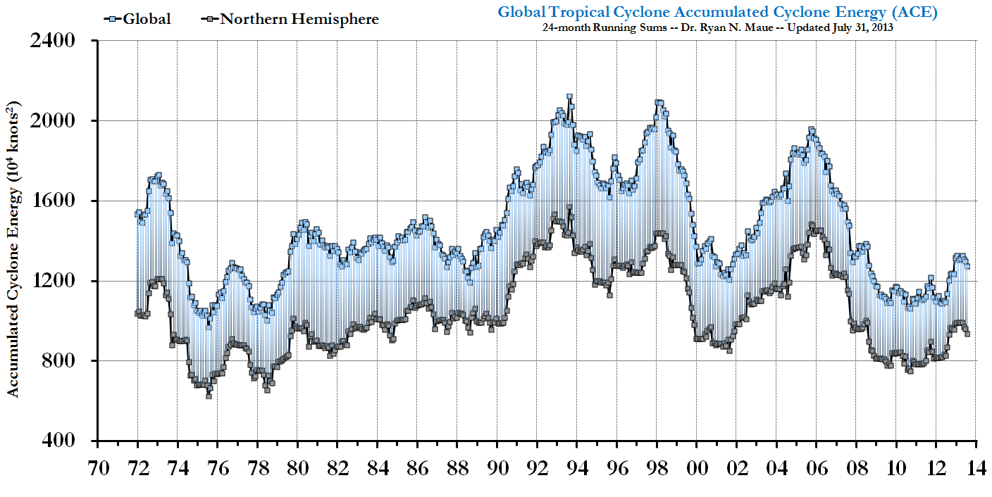
In summary, in light of the latest assessment literature and studies re-emphasizing important uncertainties, the TSD has been updated to reflect current understanding of observed changes in hurricane intensity and frequency. Refer to Volume 3 of the Response to Comments document for discussion of attribution of tropical cyclone trends.
Comment (2-91):
A commenter (3596.3) indicates the TSD ignores numerous observational studies that show Atlantic hurricanes are not getting stronger. The commenter references studies which it suggests do not indicate intensity increases in the Atlantic (Free et al., 2004; Balling and Cerveny, 2006; Latif et al., 2007).
Response (2-91):
We note the studies referenced by the commenter either do not refute that there have been increases in hurricane intensity in the Atlantic basin over the last several decades and/or rely on incomplete data. Therefore, the comment is not supported.
The commenter notes Free et al. (2004) find no consistent trend in the potential intensity of hurricanes from 1975 to 1995. This study does not analyze actual trends in actual hurricane intensity, but rather provides a theoretical measure. Importantly, the study also excludes the period 1995 to present during which hurricane activity has been elevated.
The commenter also refers to Balling and Cerveny (2006) which is a study of tropical cyclone intensification (i.e., how fast a storm strengthens after it forms) in the Atlantic basin rather than an analysis of trends in Atlantic tropical cyclone intensity over time. Though the study finds ‘no increase in a variety of [tropical cyclone] intensification indices,’ it does not contradict the assessment literature finding indicating increases in Atlantic tropical cyclone intensity over the last several decades.
Finally, the comment discusses Latif et al. (2007) who describe multi-decadal variability in Atlantic tropical cyclone activity since the late 1800s consistent with discussion in the TSD. Latif et al. (2007) indicate enhanced activity at present, which is also consistent with the TSD.
In sum, none of the studies presented refute observed increases in Atlantic tropical cyclone intensities in recent decades.
Comment (2-92):
A commenter (3747.1) argues that the TSD does not adhere to information quality guidelines under the IQA because EPA failed to consider studies, which according to the commenters, suggest that storms may decrease in intensity and become less frequent (e.g., Vecchi and Knutson, 2008). The commenter requests that EPA provide information on how scientific studies were selected to serve as basis for the TSD and how EPA dealt with studies that have come out since the release of the assessment reports.
Response (2-92):
Please see Volume 1: Section 5> of this Response to Comments document for EPA’s general response to the information quality concerns submitted during the public comment process. The science upon which the Administrator relied, including a discussion of how the literature was identified, is discussed in Section III(52 pp, 315 K, About PDF) of the Findings, and our response to comments on this can be found in Volume 1: Section 1 of the Response to Comments document. This section also describes our treatment of new and additional studies that are not incorporated into the assessment literature. EPA’s approach is fully consistent with EPA’s IQA guidelines in accordance with sound, transparent and objective scientific practices.
With regard to the commenter's reference to studies on the effects of climate change on storm intensity and frequency, please see response 2-90 in this section which reply to references or include references to several key studies specifically pertaining to this topic. We have carefully reviewed and responded to the studies submitted by the commenter (e.g., Vecchi and Knutson, 2008), along with other studies on this topic.
Comment (2-93):
A number of commenters (2750, 3136.1, 3411.1, 3596.2, 3596.3, 5058R1, 7037) suggest that evidence for increases in drought in the United States is weak or nonexistent.
Response (2-93):
To be clear, the TSD does not state that drought has, in the aggregate, increased in the United States. Indeed, Section 4(l) states that ‘[w]ith respect to drought, consistent with streamflow and precipitation observations, most of the continental United States experienced reductions in drought severity and duration over the 20th century.’ (Lettenmaier et al., 2008) We also cite Dole et al. (2008), which find: ‘It is unlikely that a systematic change has occurred in either the frequency or area coverage of severe drought over the contiguous United States from the mid-twentieth century to the present.’ However, the TSD also discusses recent increases in drought conditions in the Southwest United States, which is supported by the most recent IPCC and USGCRP assessments. Citing Lettenmaier et al. (2008), the TSD states: ‘there is some indication of increased drought severity and duration in the western and southwestern United States.’ The commenters’ broad statements about drought appear to miss this very important and well-known regional distinction.
Comment (2-94):
Several commenters (e.g., 3596.2, 3596.3, 5058R1) note that droughts in both in the United States and in some other parts of the world were more severe in the paleoclimate record (i.e., in the last several thousand years) compared to the last 100 or so years. They cite a number of studies (e.g., Seager et al., 2008; Cook et al., 2007; Cook et al., 2004; Verschuren et al., 2000) that document extreme droughts in the historic past.
Response (2-94):
EPA does not dispute that severe drought impacted the United States and other regions of the world over the last thousand years and that these droughts may have been more severe than those observed in the last 100 years in some cases. In fact, IPCC (Jansen et al., 2007) states: ‘The paleoclimatic record of northern and eastern Africa, as well as the Americas, indicate with high confidence that droughts lasting decades or longer were a recurrent feature of climate in these regions over the last 2,000 years.’ Over North America, IPCC finds the droughts over the past 2,000 years were ‘more frequent, longer and/or geographically more extensive ... than during the 20th century.’ To provide further detail in response to the comment, EPA has added the following text to Section 4(d) of the TSD: ‘The IPCC notes the trend towards drying in northern Africa and the Sahel region – with a partial recovery since 1990 – has been a common feature of climate in these regions in the paleoclimate record (Jansen et al., 2007).’ For the discussion of U.S. drought, EPA has added in Section 4(l): ‘The IPCC noted, however, based on paleoclimate studies, that over the past 2,000 years drought in North America was more frequent, longer and/or geographically more extensive ... than during the 20th century (Jansen et al., 2007).’
Comment (2-95):
One commenter (3596.2) notes that while heavy precipitation has increased, these increases have been precisely proportional to the increase in average rainfall, citing Michaels et al. (2004). The commenter takes issue with the statement in the TSD that increases in heavy precipitation have occurred ‘even in those [land regions] where there has been a reduction in total precipitation amount.’ The commenter concludes that ‘there was no general indication of a trend towards a more extreme precipitation climate in the U.S., allowing for the fact that precipitation itself has increased.’
Response (2-95):
EPA reviewed the TSD in light of the comment and submitted literature, and we disagree with the commenter’s assertions. Section 4(l) of the TSD summarizes the assessment literature on this subject, and states that ‘[t]he increase in the frequency and intensity of heavy downpours was responsible for most of the observed increase in overall precipitation during the last 50 years (Karl et al., 2009).’
We note that the study by Michaels et al. (2004) was assessed by CCSP (Kunkel et al., 2008), which states: ‘the amount of precipitation falling in the heaviest 1% of rain events increased by 20% during the 20th century, while total precipitation has increased by 7%’ (Groisman et al., 2004). Although the exact character of those changes have been questioned (e.g., Michaels et al., 2004), it is highly likely that in recent decades extreme precipitation events have increased more than light to medium events.’ EPA agrees with the assessment of Kunkel et al. (2008) which was reinforced by the statements on the issue in Karl et al. (2009), so no change to the TSD is required.
Comment (2-96):
One commenter (3394.1) takes issue with the TSD statement that ‘[i]t is likely that there have been increases in the number of heavy precipitation events (e.g., 95th percentile) within many land regions, even in those where there has been a reduction in total precipitation amount, consistent with a warming climate and observed significant increasing amounts of water vapor in the atmosphere.’ The commenter asserts that the statement is a guess, not an observation.
Response (2-96) :
This TSD statement, which is found in Section 4(k), ‘Global Extreme Events,’ is taken directly from IPCC (Trenberth et al., 2007). It is not a guess but an expert judgment (with the choice of the word ‘likely’ suggesting greater than 66% probability) based on considerable observational evidence. The IPCC bases its statement on much of the following observational evidence:
- In Europe, there is a clear majority of stations with increasing trends in the number of moderately and very wet days during the second half of the 20th century.
- For the contiguous United States, studies cited by IPCC found statistically significant increases in heavy and very heavy precipitation, with much of this increase during the last three decades of the 20th century.
- Despite a decrease in mean annual rainfall, an increase in the faction from heavy events was inferred for large parts of the Mediterranean.
- In South Africa, Siberia, central Mexico, and Japan, an increase in heavy precipitation was observed while total precipitation and/or the frequency of days with an appreciable amount of precipitation (wet days) either unchanged or decreasing.
- Averaged over central and southern Asia, a slight indication of disproportionate change in the precipitation extremes compared with the total amounts is seen.
- In the Indian sub-continent, IPCC cites a study that finds two-thirds of all considered time series exhibit increasing trends in indices of precipitation extremes.
- Analysis of global land areas concludes that the percentage contribution to total annual precipitation from very wet days (upper 5%) is greater in recent decades than in earlier decades. Observed changes in intense precipitation for more than one half of the global land area indicate an increasing probability of intense precipitation events beyond that expected from change in the mean for many extratropical regions.
Given the scope and nature of the observational evidence, and the characterization of uncertainty that accompanies this conclusion, we conclude that the statement in the TSD is reasonable and sound, and see no reason to revise it.
See Volume 1 of this Response to Comments document for responses on comments related to the characterization of uncertainty in the assessment literature upon which the TSD relies.
Comment (2-97):
A commenter (3596.3) contends the TSD has conflicting statements on heavy precipitation and flooding. The comment notes the TSD states: ‘increases in heavy precipitation events have been linked to increase in flooding’ and ‘significant trends in floods and in evaporation and evapotranspiration have not been detected globally.’
Response (2-97):
We disagree that these statement are inconsistent because they are saying different things. The first statement is noting a relationship between heavy precipitation and flooding, which is difficult to dispute. The second statement is simply referring to the IPCC’s (Rosenzweig et al., 2007) assessment of global trends in flooding.
Comment (2-98):
Several commenters (e.g. 3136.1, 3145.1, 3411.1) indicated there have been no long-term increases in strong U.S. East Coast winter storms (sometimes referred to as nor’easters).
Response (2-98):
The TSD does not suggest long-term increases in strong U.S. winter storms, and we agree with commenters that increasing trends have not been detected in U.S. East Coast winter storm intensity. Section 4(l) of the TSD states: ‘Karl et al. (2008) indicate a northward shift in the tracks of strong low-pressure systems (also known as mid-latitude storms and/or extratropical cyclones) in both the North Atlantic and North Pacific over the past fifty years with increases in storm intensity noted in the Pacific (data inconclusive in the Atlantic).’ In other words, Karl concludes that the storm tracks appear to be shifting northward, but does not find evidence that intensity is increasing in the Atlantic or along the East Coast. We conclude that the TSD accurately reflects the assessment literature on this issue.
Comment (2-99):
One commenter (3596.2) suggests the TSD does not reflect current state of knowledge with respect to non-tropical storms (also referred to as extratropical cyclones, low pressure systems, and mid-latitude storms). The commenter notes:
EPA background documents did not include Hanna et al. (2008), who found ‘there is little evidence that the mid-to late nineteenth century was less stormy than the present and there is no sign of a sustained enhanced storminess signal associated with ‘global warming.’ Similarly, Matulla et al. (2007) found no trends in daily wind strength (a measure of storminess) in Europe back to the late 19th century. Similarly, over a longer period and using a direct measure of storm intensity (frequency of low barometric pressure), Barring and von Storch (2004), which is not cited by the CCSP, found no evidence of any systematic change in non-tropical storm intensity for over two centuries.
Response (2-99):
We have reviewed the TSD in light of the comment and literature provided, and find that the characterization in the TSD is reasonable and sound. Regarding Northern Hemisphere trends in non-tropical storms (also known as low pressure systems or extratropical storms), Section 4(k) of the TSD, citing IPCC, states: ‘Trenberth et al. (2007) find there haslikely been a net increase in frequency and intensity of strong low-pressure systems (also known as mid-latitude storms and/or extratropical cyclones) over Northern Hemisphere land areas, as well as a poleward shift in track since about 1950.’ Trenberth et al. (2007) reference numerous studies, which have documented such changes to draw this conclusion.
We found that the studies cited by the commenter are broadly consistent with Trenberth et al. (2007) as reflected in the TSD, with some minor exceptions. Though Hanna et al. (2008) do not attribute recent trends in storminess to global warming, they do find recent increases in intensity (for northwestern Europe and the northern North Atlantic), stating: ‘Our findings are much in line with those of previous studies that pick up a general increase in North Atlantic cyclonicity and storminess between the 1960s and 1990s although this varies by region.’ Matulla et al. (2007) analyze storminess in central Europe and also find evidence for increasing storminess from the 1960s to 1990s, though they show recent values show a return to average or calm conditions.
Barring and von Storch (2004) examined storminess trends in Scandinavia. They identified a period of enhanced storminess from the 1980s to mid-1990s but conclude that there are no robust signs of any long-term trend in the storminess indices. We note that this study analyzed a relatively small geographic area and was cited and assessed by IPCC (Trenberth et al., 2007) even if not cited by CCSP (as indicated by the commenter).
Though it was not cited by the commenter, we have also reviewed the recent study by Wang et al. (2009), which finds that ‘The atmospheric storminess has increased in boreal winter over the past half century in the high-latitudes of the northern hemisphere (especially the northeast North Atlantic), and has decreased in more southerly northern latitudes.’
Thus, we conclude from our review of the studies on this topic that there is general support for the conclusions of the IPCC and CCSP assessments that detection of long-term changes in cyclone measures is hampered by incomplete and changing observing systems, and that there is substantial decadal variability in extratropical cyclone trends. Nonetheless, to provide further clarification on this, we have added the following language to the TSD to reflect these conclusions: ‘detection of long-term changes in cyclone measures is hampered by incomplete and changing observing systems. They [Trenberth et al., 2007] also note longer records for the northeastern Atlantic suggest that the recent extreme period may be similar in level to that of the late 19th century.’
Comment (2-100):
A number of commenters (e.g., 0700.1, 1312, 2750, 3145.1, 3411, 11000) noted no recent trends in the severity/frequency of thunderstorms and tornadoes either globally or in the United States.
Response (2-100):
Information on trends in thunderstorms or tornadoes was not included in the version of the TSD released in April 2009 with the Proposed Finding, but we have revised the TSD and now provide such information in Sections 4(k) and 4(l). For global trends in thunderstorms, tornadoes, and related phenomena (e.g., hail), EPA has included the following statement from IPCC’s Fourth Assessment Report in Section 4(k): ‘There is insufficient evidence to determine whether trends exist ... in small-scale phenomena such as tornadoes, hail, lightning and dust-storms.’ For trends in the United States, EPA cites Kunkel et al. (2008) in Section 4(l): ‘There is no evidence for a change in the severity of tornadoes and severe thunderstorms, and the large changes in the overall number of reports make it impossible to detect if meteorological changes have occurred.’
Comment (2-101):
Several commenters (e.g., 3145.1, 3187.3, 3596.2) note that there is no indication that extreme heat or record heat is increasing and that the most severe heat waves in the United States occurred during the 1930s.
Response (2-101):
We disagree that extreme heat has not increased in recent decades. CCSP (Kunkel et al., 2008) finds: ‘since 1950, the annual percent of days exceeding the 90th, 95th, and 97.5th percentile thresholds for both maximum (hottest daytime highs) and minimum (warmest nighttime lows) temperature have increased when averaged over all of North America. This information has been added to Section 4(l) of the TSD to clarify. We further note that a recent study by Meehl et al. (2009) find the ratio of record high temperatures to record low temperatures has substantially increased since the late 1970s, primarily due to fewer record low temperatures.
EPA agrees, however, that the most severe heat waves on record in the United States occurred during the 1930s. The TSD states that ‘the heat waves of the 1930s remain the most severe in the U.S. historical record.’ For responses to comments on the human health effects of heat, please refer to Volume 5.
Comment (2-102):
Several commenters (e.g., 3136.1 and 3596.2) assert there has been no long-term trend in heat waves or cold spells in the United States though there are trends within shorter time periods in the overall record.
Response (2-102):
The commenters did not provide specific information to support their assertion, and it is not possible to evaluate its validity since they did not define the period they were considering. The TSD, in Section 4(l), cites CCSP (Kunkel et al., 2008), which finds a highly statistically significant increase in the number of U.S. heat waves (defined as warm spells of four days in duration with mean temperature exceeding the threshold for a 1 in 10 year event) for the period 1960 to 2005. We maintain that 45 years constitutes a long-term trend, though we note Kunkel et al. (2008) state there is no trend over the entire 1895-2005 period (largely due to the heat waves in the 1930s, referred to in response 2-101).
We also note that Kunkel et al. (2008) refer to the study of Peterson et al. (2008) which finds the annual number of warm spells (defined as at least three consecutive days above the 90th percentile threshold done separately for maximum and minimum temperature) averaged over all of North America has increased since 1950. These findings serve as the basis for the CCSP conclusion (Karl et al., 2008) that ‘the number of heat waves (extended periods of extremely hot weather) has been increasing over the past 50 years.’
With respect to cold spells in the United States, Kunkel et al. (2008) find some evidence of a downward linear trend in cold waves (extended periods of cold) for the 1895-2005 period, but note the trend is not statistically significant, largely owing to multi-decadal variability. They state cold waves show a decline in the first half of the 20th century, then a large spike during the mid-1980s, then a decline in the last two decades. They then note the very recent period from 1998 to 2007 exhibited fewer severe cold snaps than for any other 10-year period in the historical record dating back to 1895.
Accordingly, though we do not agree with the commenters’ statement that there is unequivocally ‘no long-term trend’ in this measure, we do concur that the most robust trends are found within shorter time periods. The TSD has been updated to provide more detail about cold spell variability and trends.
Comment (2-103):
A commenter (3596.3) claims that observational evidence does not support the TSD’s statement that changes in the frequency and amplitude of certain weather patterns might also trigger other processes such as El Niño that lead to abrupt climate change. The commenter presents a list of studies to support this assertion.
Response (2-103):
We disagree that we do not provide observational evidence suggestive of a link between El Niño and abrupt climate change. The TSD includes the following statement from the assessment literature (Clark et al., 2008): ‘ENSO [El Niño Southern Oscillation] has important linkages to patterns of tropical sea surface temperatures, which historically have been strongly tied to drought, including ‘megadroughts’ that likely occurred between 900 and 1600 A.D. over large regions of the southwestern United States and Great Plains.’
We further note that list of studies provided by the commenter do not refute the links between drought and El Niño but rather emphasize the uncertainty in modeling El Niño. We agree that modeling El Niño is
difficult. In fact, citing the assessment literature (Clark et al., 2008) in the TSD, we state: ‘models may not correctly represent the ENSO [El Niño Southern Oscillation] patterns of tropical SST [sea surface
temperature] change.’
Comment (2-104):
A commenter (3596.3) indicates EPA ‘overlooked’ a number of studies that present an opposite point of view on extreme high sea level. The comment presents a list of studies to support its assertion.
Response (2-104):
Summarizing the assessment literature, the TSD states: ‘There is evidence for an increase in extreme high sea level since 1975 based upon an analysis of 99th percentiles of hourly sea level at 141 stations over the globe (Bindoff et al., 2007).’ The studies provided by the commenter do not refute this finding. Six of the seven studies submitted provide sea level data from individual locations or small regions, which collectively offer no insight on global trends. The other study does not even provide data pertaining to sea level.
2.6 Changes in Physical and Biological Systems
2-105 | 2-106 | 2-107 | 2-108 | 2-109 | 2-110 | 2-111 | 2-112 | 2-113 | 2-114 | 2-115
Comment (2-105):
A few commenters from Canada (3598.1) and Alaska (3609.2) express their support for the Findings and note their observations of perceived global warming impacts in Arctic climates (e.g., reduced or thinning sea ice). Many commenters (e.g., 1018.1, 1117.1, 1118.1, 1156.1, 3455.1, 3642, 4184, 4249, 6735, 6936) state their support for the Findings, noting observations of melting ice caps in polar regions as one of the environmental effects of climate change.
Response (2-105):
EPA agrees the Arctic is warmer at a faster rate than the global average and that Arctic sea ice is rapidly declining. For additional discussion of Arctic temperatures, refer to the TSD Section 4(b) and for discussion of Arctic sea ice, refer to TSD Section 4(i)(210 pp, 2.5 M, About PDF). See the Findings, Section IV.B(52 pp, 315 K, About PDF), ‘The Air Pollution Is Reasonably Anticipated to Endanger Both Public Health and Welfare,’ for our response to comments on how the Administrator weighed the scientific evidence underlying her endangerment determination.
Comment (2-106):
A commenter (3283.1) questions EPA’s conclusion that observed warming and associated impacts like earlier onset of spring can be attributed to human actions. The commenter states that literature not cited by EPA identifies large uncertainty regarding the cause of observed earlier onset of spring. As an example, the commenter cites a study by White et al. (2009) which assessed the suite of methods used to estimate the onset of spring and found an average difference of 60 days across methods for the time period 1982-2006. The commenter quotes the article’s conclusion that
Trend estimates from the Start of Spring (SOS) methods as well as measured and modeled plant phenology strongly suggest either no or very geographically limited trends towards earlier spring arrival, although we caution that, for an event such as SOS with high interannual variability, a 25-year SOS record is short for detecting robust trends. Increased greenhouse warming since the late 20th century would seem to argue for increased, not decreased, shifts in spring during our study period, indicating that processes such as succession, changes in community structure, land management, or disturbance may be more important than previously recognized. Seasonal temperature changes may also be linked to a trend reversal in SOS in the early 1990s.
Response (2-106):
See Volume 3 of this Response to Comments document for our responses to general comments on the issue of attributing observed temperature increases to anthropogenic forcing. Regarding attribution of associated impacts like earlier onset of spring, we discuss in Section 5 of the TSD how the IPCC (Rosenzweig et al., 2007) reviewed a number of studies that linkedchanges in some physical and biological systems directly to anthropogenic climate change. The IPCC concluded that the observed changes in physical and biological systems ‘likely cannot be explained entirely due to natural variability or other confounding non-climate factors’ (Rosenzweig et al., 2007).
EPA carefully reviewed the referenced study and finds that the conclusions of White et al. (2009) regarding the potential for multiple factors to influence earlier spring arrival are generally consistent with the information presented in the TSD. We describe in Section 5(b) of the TSD the importance of considering climate variability and non-climate drivers (e.g., land-use change, habitat fragmentation) in order to make robust conclusions about the role of anthropogenic climate change in affecting biological and physical systems.
However, the conclusions of White et al. (2009) regarding the lack or weakness of a trend toward earlier spring arrival are inconsistent with the conclusions of the scientific assessment literature. As shown in the quote provided by the commenter, the study authors themselves acknowledge that a 25 year record is short for detecting robust trends. As summarized in the TSD, IPCC (Rosenzweig et al., 2007) states with very high confidence that the majority of studies of regional climate effects on terrestrial species reveal consistent responses to warming trends across the Northern Hemisphere. These responses are well-documented and include changes in the earlier onset of spring events, migration, and lengthening of the growing season, which in turn affect the seasonal timing of species’ life cycle events (that is, phenological changes). Section 14 of the TSD mentions several studies reviewed by the IPCC (Field et al., 2007) documenting observations of climate change effects on plant and animal phenology. Given that there are several lines of evidence in specific regions which suggest changes in phenology correlated with climate, we find that the TSD’s discussion of this topic is accurate and appropriately reflects the body of scientific literature.
Comment (2-107):
A commenter (3747.1) cites Parmesan (1996) as a ‘relevant credible rebuttal study’ meant to rebut the conclusions of the literature cited in the TSD. The commenter provides no other associated comments.
Response (2-107):
The commenter did not present specific critiques of the information in the TSD, nor describe how this study was to be reviewed and considered by EPA. We reviewed Parmesan (1996) and note that its discussion of climate change effects on species’ ranges is consistent with the scientific assessment literature as summarized in the TSD; in fact, it is cited by the IPCC (Field et al. 2007). We therefore find that the TSD’s discussion of this topic is accurate and appropriately reflects the body of scientific literature.
Comment (2-108):
A commenter (9733) indicates that snow seasons are not shorter. The past two years, the commenter states, have been bumper seasons for Victoria’s snow resorts; this year could be just as good, with snow already falling in New South Wales and Victoria this past week.
Response (2-108):
The commenter’s points appear to be based on personal observation and conjecture over a very short time period in one particular location. They not supported by the scientific literature, and EPA notes that an undocumented and unreferenced description regarding two years of snowfall in one location is not evidence that snow seasons are not shorter. Furthermore, we note that the locations described by the commenter, New South Wales and Victoria, are in Australia, not the United States. The assessment literature provides robust evidence that decreasing snow season lengths have been observed globally and in the United States (Christensen et al., 2007; Field et al., 2007; Lettenmaier et al., 2008). Regarding the issue of snow season length, the TSD makes the following conclusions:
Consistent with these findings, Lettenmaier et al. (2008) note a trend toward reduced mountain snowpack, and earlier spring snowmelt runoff peaks across much of the western U.S.
Snow season length and snow depth are very likely to decrease in most of North America as illustrated in Figure 6.11, except in the northernmost part of Canada where maximum snow depth is likely to increase (Christensen et al., 2007).
Comment (2-109):
A commenter (11241) refers to the rapid decline of Arctic sea ice as an indicator of one of many tipping points in the climate system and advocates strong action on climate change in response. Another commenter (3344.2) refers to rapid warming in the Arctic, the decline of Arctic sea ice, and many related impacts as justification for EPA’s endangerment finding.
Response (2-109):
EPA agrees that the rapid pace of changes occurring in the Arctic is well-supported in the scientific literature and documented in the TSD. We note, as stated in the Executive Summary of the TSD: ‘This document provides technical support for the endangerment analysis concerning greenhouse gas (GHG) emissions that may be addressed under the Clean Air Act. This document itself does not convey any judgment or conclusion regarding the question of whether GHGs may be reasonably anticipated to endanger public health or welfare, as this decision is ultimately left to the judgment of the Administrator.’ Thus, this volume of the Response to Comment document provides EPA’s responses to technical issues raised regarding the TSD. See Volume 9 for EPA’s responses on the Administrator’s determination, in general and with respect to climate impacts. See the Findings, Section IV.B(52 pp, 315 K, About PDF), ‘The Air Pollution Is Reasonably Anticipated to Endanger Both Public Health and Welfare,’ for our response to comments on how the Administrator weighed the scientific evidence underlying her endangerment determination.
Comment (2-110):
Several commenters (0303, 0364, 0591, 3432.1, 3596.2) indicate that global sea ice area has not changed significantly (or even risen) since 1979.
Response (2-110):
In the TSD, EPA does not address global sea ice area as an indicator of climate change, because it is neither discussed nor documented in this context in IPCC or CCSP. Instead, EPA addresses the trends in sea ice separately for the Arctic and Antarctica, because of evidence that different process may be at work in the northern and southern hemispheres. EPA has reviewed the long-term time series of global sea ice area provided by the University of Illinois - Champaign Arctic Climate Research Group and agrees with its conclusion that there has been little change in global sea ice since 1979 (Arctic Climate Research Group, 2009a: http://arctic.atmos.uiuc.edu/cryosphere/IMAGES/global.daily.ice.area.withtrend.jpg). The Arctic Climate Research Group documented this in a public statement early in 2009 (see Arctic Climate Research Group, 2009b: http://arctic.atmos.uiuc.edu/cryosphere/global.sea.ice.area.pdf(1 pp, 254 K, About PDF)). In that statement, however, the research group noted ‘in the context of climate change, GLOBAL sea ice area may not be the most relevant indicator,’ alluding to the fact that different processes influence ice in the Northern and Southern Hemispheres. EPA concurs with this statement, and our approach in Section 4(i) of the TSD reflects this.
Comment (2-111):
Multiple commenters (e.g., 0430, 0498, 0539, 3136.1, 3224, 3373, 9733) refer to the fact that Antarctica has been gaining ice since 1979.
Response (2-111):
Based on our review of the literature, EPA concludes that Antarctica has gained sea ice since 1979, but has not gained land ice.
In the April version of the TSD, EPA stated: ‘Antarctic sea ice extent shows no statistically significant average trends according to IPCC (2007d). However, the U.S. National and Snow and Ice Data Center [NSIDC] states that Antarctic sea ice underwent a slight increase from 1979 to 2007 (NSIDC, 2009).’ EPA acknowledges these two sentences, taken together, may confuse the reader. And we are also aware of updated data from NSIDC. So we have revised the TSD to provide more clarity. It now reads: ‘For the period 1979-2008, Antarctic sea ice underwent a not statistically significant increase of 0.9% (about 100,000 km2; 42,000 mi2) per decade (NSIDC, 2009).’
Though we concur there has been a net increase in Antarctic sea ice, we disagree that Antarctica has gained land ice since 1979. CCSP (Clark et al., 2008) report that the land area of Antarctica is losing ice overall, though in certain regions ice is thickening. We are also aware of a recent study (Chen et al., 2009) that quantifies changes in land ice over Antarctica spanning the period April 2002 to January 2009 and estimates a total loss of 190 ? 77 Gt per year, with 132 ? 26 Gt per year coming from West Antarctica. Notably, in contrast with prior studies, this study suggests that East Antarctica is losing mass, mostly in coastal regions, at a rate of -57 ? 52 Gt per year, apparently caused by increased ice loss since the year 2006.
Comment (2-112):
Several commenters note Arctic sea ice has rapidly recovered since reaching its 2007 minimum (0364, 0498, 0591, 3446.1).
Response (2-112):
EPA does not agree with the commenters’ portrayal of this situation. EPA clearly states in Section 4(i) of the TSD that September Arctic sea ice extent reached a minimum in 2007, its second lowest on record in 2008, and third lowest on record in 2009. The implication, therefore, is that there has been some recovery since the minimum. The key conclusion however, is not that there has been a very modest recovery, but rather that the 2009 September low was still 1.68 million square kilometers (649,000 square miles) below the 1979 to 2000 September average (NSIDC, 2009b: http://nsidc.org/news/press/20091005_minimumpr.html). The TSD has been updated to discuss the 2009 minimum sea ice extent, reflecting the most current and complete information on Arctic sea ice trends. It also includes the finding that the total annual Arctic sea ice extent has been declining at the rate of 4.1% (about 500,000 square kilometers; 193,000 square miles) per decade for the 1979-2008 (NSIDC, 2009a: http://nsidc.org/seaice/characteristics/difference.html), which updates the finding from the TSD that ‘satellite data since 1978 show that annual average Arctic sea ice extent has shrunk by 2.7 +/- 0.6% per decade.’
Comment (2-113):
Several commenters indicate that Arctic sea ice reached comparably low levels prior to satellite monitoring, specifically mentioning the late 1950s (3317.1, 3729.8), the 1800s (3729.8) and when the Vikings established settlements in Greenland (2750).
Response (2-113):
The commenters provide anecdotal evidence and historical accounts describing thin Arctic sea ice prior to the satellite era. This information does not provide the necessary data for EPA to assess their validity, and it conflicts with existing assessment literature cited by IPCC and CCSP. IPCC cites numerous studies which, to the extent possible, examine trends in Arctic sea ice dating back as far the late 1800s. All of the studies document declining ice extent during the latter decades of the 20th century, and the decline begins prior to the satellite era. The IPCC notes that there are problems with homogeneity of the pre-satellite data (with quality declining further back in history) and with the disparity in spatial scales represented by each. For example, IPCC cites Russian data (Polyakov et al., 2003), which indicate anomalously little ice during the 1940s and 1950s, but also Nordic Sea data (Vinje, 2001) indicating anomalously large extent at that time. The CCSP report Past Climate Variability and Change in the Arctic and at High Latitudes, after an extensive survey of the relevant literature, concludes: ‘Ice cover in the Arctic began to diminish in the late 19th century and this shrinkage has accelerated during the last several decades. Shrinkages that were both similarly large and rapid have not been documented over at least the last few thousand years, although the paleoclimatic record is sufficiently sparse that similar events might have been missed’ (Alley et al., 2009).
In response to this comment, EPA has added language to the TSD to provide additional detail about historical Arctic sea ice information. This discussion in Section 4(i) now reads: ‘Ice cover in the Arctic began to diminish in the late 19th century, and this shrinkage has accelerated during the last several decades. Shrinkages that were both similarly large and rapid have not been documented over at least the last few thousand years, although the paleoclimatic record is sufficiently sparse that similar events might have been missed (Alley et al., 2009).’
Comment (2-114):
A number of commenters (e.g., 3535, 3596.3, 3722R126) report that the TSD’s portrayal of trends in glacier mass balance is inaccurate or invalid. They cite examples of glaciers that are growing rather than retreating, as well as studies that document such trends. They also note there has been no recent acceleration in the rate of recession where glaciers continue to recess.
One commenter (3535) citing NIPCC (Singer and Idso, 2009), indicates sparse data exists about glaciers. Similarly, a commenter (3596.3) notes that very few glacier data exist, referring to a study that indicates only 42% of glaciers have been inventoried to any degree (Kieffer et al., 2000) and only ‘a tad over 200’ glaciers for which mass balance data exist (Braithewaite and Zhang, 2000). The commenter notes that Braithewaite and Zhang state that ‘many glacierized regions of the world remain unsampled, or only poorly sampled.’ The commenter refers to Braithwaite (2002) which notes that ‘there is no common or global trend of increasing glacier melt in recent years.’
Response (2-114):
EPA strongly disagrees that the TSD’s portrayal of a general decline in glaciers is inaccurate or invalid. The TSD does not say that all glaciers are receding and states that the rate of glacier melt is variable. Though we agree a relatively small percentage of the world’s glaciers are sampled as noted in the studies referenced, it does not impact our confidence in the general trend as the overwhelming majority of glaciers sampled are declining. In addition, there is evidence for recent acceleration in glacier decline.
In Section 4(i), the TSD states ‘Mountain glaciers ... have declined on average in both hemispheres’ where ‘on average’ implies changes of varying signs and rates. Though the studies cited by IPCC (e.g., Oerlemans, 2005; Dyurgerov and Meier, 2005) demonstrate widespread large-scale retreat of glacier tongues since the 1800s and mass losses since the 1960s, when these measurements began, it also notes high spatial and temporal variability in glacier trends. For example, it discusses glaciers along the coast of Norway and in the New Zealand Alps, which advanced in the 1990s and started to shrink around 2000. It also notes that whereas glaciers in the high mountains of Asia have generally shrunk, several high glaciers in the central Karakoram are reported to have advanced and/or thickened at their tongues.
For additional clarification, we have revised Section 4(i) of the TSD to note the relatively small number of sampled glaciers and provide additional detail on glacier trends. It now states:
Though the studies cited by the IPCC (in Lemke et al., 2007) demonstrate widespread large-scale retreat of glacier tongues since the 1800s and mass losses since the 1960s (when mass loss measurements began), IPCC cautions records of directly measured glacier mass balances are few, and that there is high spatial and temporal variability in glacier trends. For example, it discusses glaciers along the coast of Norway and in the New Zealand Alps that advanced in the 1990s and started to shrink around 2000. It also notes that whereas glaciers in the high mountains of Asia have generally shrunk, several high glaciers in the central Karakoram are reported to have advanced and/or thickened at their tongues.
Regarding the issue of acceleration, we note the USGCRP assessment (Karl et al., 2009) finds:
Glaciers have been retreating worldwide for at least the last century, and the rate of retreat has increased in the last decade. Only a few glaciers are actually advancing (in locations that were well below freezing and where increased precipitation has outpaced melting). The total volume of glaciers on Earth is declining sharply.
In addition, a recent study (Zemp et al., 2009) reviewing world glacier observations over the past six decades (1946-2006) finds: ‘The available data from the six decades indicate a strong ice loss as early as the 1940s and 1950s followed by a moderate mass loss until the end of the 1970s and a subsequent acceleration that has lasted until now’
This acceleration is also noted in a recent study by Braithwaite (2009) which reports: ‘30 year series from 30 glaciers confirm a recent (1996-2005) trend to very negative mass balance after two decades of nearly zero mass balance.’ This finding from Braithwaite clearly updates the finding referenced in the Braithwaite (2002) study referenced by the commenter which noted no global trend of increasing glacier melt in recent years (the study period ended in 1995).
In light of this evidence for acceleration from the USGCRP assessment and these additional studies, we have added the italicized text to this statement in section 4(i) of the TSD:
Mountain glaciers and snow cover have declined on average in both hemispheres with evidence of acceleration in glacier decline in the last decade (Karl et al., 2009).
In sum, though a relatively small percentage of the world’s glaciers are sampled and there is evidence for spatial and temporal variability, the assessment literature is clear that most observed glaciers are declining and that the rate of decline has increased recently.
For discussion of attribution of glacier trends, please refer to Volume 3 of this Response to Comments document.
Comment (2-115):
A commenter (3729.7) posits that the trends in western North America snowpack are biased due to the start date of the analysis, which was 1950. The comment suggests that time series in the supporting analysis begins at a time when snowfall was very high in the Pacific Northwest and that the trend would differ if the start date was altered. The comment does not specifically address the discussion of this issue in the TSD.
Response (2-115):
The April 2009 version of the TSD does not address the magnitude of the western North America snowpack trend, nor does it display the time series in question. It states: ‘Lettenmaier et al. (2008) note a trend toward reduced mountain snowpack, and earlier spring snowmelt runoff peaks across much of the western U.S.’ This statement is supported by the studies cited by Lettenmaier et al. (e.g., Mote et al., 2005; Hamlet et al., 2005). The findings of newer studies reviewed by EPA (Casola et al., 2009; Stoelinga et al., 2009 manuscript submitted to J. Climate) analyzing snowpack trends in the Cascade Mountains of the Pacific Northwest do not provide evidence to warrant any change to the above statement from the TSD. In fact, Stoelinga et al. (2008,) report: ‘Cascade spring snowpack declined 23% during 1930-2007. This loss is nearly statistically significant at the 95% level.’ Accordingly, EPA does not believe the TSD statement requires modification. However, these studies do indicate that shorter-term decadal-scale trends are quite sensitive to the start date of the analysis, which is consistent with the concern expressed in this comment. For example, Casola et al. (2009) write: ‘The sensitivity of the trends to the choice of period of record is underscored by sharply contrasting results of Mote et al. (2008), who reported losses of up to 35% in springtime snow-water equivalent (SWE) at stations in the Pacific Northwest for a variety of periods beginning around the mid-twentieth century and ending in 2006, and Stoelinga et al. (2009, manuscript submitted to J. Climate), who found little, if any, trend in SWE at stations in the same region from 1977 to 2006.’ The decadal variability in western snowpack trends has implications for the attribution of these trends to climate change and is further discussed in Volume 3 of this Response to Comments document.
References
Aeschbach-Hertig, W. (2007). Rebuttal of ‘On global forces of nature driving the Earth’s climate. Are humans involved?’ by L.F. Khilyuk and G.V. Chilingar. Environ Geol 52:1007-1009. doi:10.1007/s00254-006-0519-3.
Akasofu, S.I. (2007) Is the Earth still recovering from the ‘Little Ice Age’? International Arctic Research Center, University of Alaska Fairbanks. http://www.iarc.uaf.edu/highlights/2007/akasofu_3_07/Earth_recovering_from_LIA_R.pdf(23 pp, 10.7 M, About PDF).
Alaska Climate Research Center (2005). Temperature change in Alaska 1977-2008. http://climate.gi.alaska.edu/ClimTrends/Change/7708Change.html. Accessed December 5, 2009.
Arctic Climate Research Group (2009a). Global sea ice area: 1979-present. http://arctic.atmos.uiuc.edu/cryosphere/IMAGES/global.daily.ice.area.withtrend.jpg. Accessed December 5, 2009.
Arctic Climate Research Group (2009b). Public statement on global sea ice area since 1979,http://arctic.atmos.uiuc.edu/cryosphere/global.sea.ice.area.pdf(1 pg, 254 K, About PDF). Accessed December 5, 2009.
Balling Jr., R.C., and R.S. Cerveny (2006). Analysis of tropical cyclone intensification trends and variability in the North Atlantic Basin over the period 1970-2003. Meteorological and Atmospheric Physics 93:45-51.
Barring, L., and H. von Storch (2004). Scandinavian storminess since about 1800. Geophys. Res. Lett. 31: L20202. doi:10.1029/2004GL020441.
Beck, E.-G. (2007). 180 years of atmospheric CO2 analysis by chemical methods. Energy & Environment 18:259-282.
Bengtsson, L., K. I. Hodges, M. Esch, N. Keenlyside, L. Kornblueh, J.-J. Luo, and T. Yamagata (2007). How may tropical cyclones change in a warmer climate. Tellus A 59(4):539-561.
Braithwaite, R.J., and Y. Zhang (2000). Relationships between interannual variability of glacier mass balance and climate.Journal of Glaciology 45:456-462.
Braithwaite, R.J. (2002). Glacier mass balance: The first 50 years of international monitoring. Progress in Physical Geography 26:76-95.
Braithwaite, R.J. (2009). After six decades of monitoring glacier mass balance we still need data but it should be richer data. Ann. Glaciol. 50(50):191-197.
Brohan, P., J.J. Kennedy, I. Harris, S.F.B. Tett, and P.D. Jones (2006). Uncertainty estimates in regional and global observed temperature changes: a new dataset from 1850. J. Geophysical Research 111: D12106. doi:10.1029/2005JD006548.
Buntgen, U., D. Frank, D. Nievergelt, and J. Esper (2006). Summer temperature variations in the European Alps, AD 755-2004. Journal of Climate 19:5606-5623.
Carlin, A. (2009). Proposed NCEE Comments on Draft Technical Support Document for Endangerment Analysis for Greenhouse Gas Emissions under the Clean Air Act.
Cazenave, A., et al. (2009). Sea level budget over 2003-2008: A reevaluation from GRACE space gravimetry, satellite altimetry and Argo. Global Planetary Change 65:83-88.
CCSP (2007). The First State of the Carbon Cycle Report (SOCCR): The North American Carbon Budget and Implications for the Global Carbon Cycle. A Report by the U.S. Climate Change Science Program and the Subcommittee on Global Change Research [King, A.W., L. Dilling, G.P. Zimmerman, D.M. Fairman, R.A. Houghton, G. Marland, A.Z. Rose, and T.J. Wilbanks (eds.)]. Asheville, NC: National Oceanic and Atmospheric Administration, National Climatic Data Center. 242 pp.
Casola, J.H., et al. (2009). Assessing the impacts of global warming on snowpack in the Washington Cascades. Journal of Climate 22(May).
Chang, E. K. M., and Y. Guo (2007), Is the number of North Atlantic tropical cyclones significantly underestimated prior to the availability of satellite observations?, Geophys. Res. Lett., 34, L14801, doi:10.1029/2007GL030169.
Chen, J.L., C.R. Wilson, D. Blankenship, and B.D. Tapley (2009). Accelerated Antarctic ice loss from satellite gravity measurements. Nature Geoscience. doi:10.1038/ngeo694.
Christy, J.R., W.B. Norris, and R.T. McNider (2009). Surface temperature variations in East Africa and possible causes. J. Clim. 22. doi:10.1175/2008JCLI2726.1.
Christy, J.R., W.B. Norris, K. Redmond, and K. Gallo (2006). Methodology and results of calculating central California surface temperature trends: Evidence of human-induced climate change? J. Climate 19:548-563.
Church, J.A., N.J. White, R. Coleman, K. Lambeck, and J.X. Mitrovica (2004). Estimates of the regional distribution of sea level rise over the 1950-2000 period. Journal of Climate 17:2609-2625.
Chylek, P., C.K. Folland, G. Lesins, M.K. Dubey, and M. Wang (2009). Arctic air temperature change amplification and the Atlantic Multidecadal Oscillation. Geophys. Res. Lett. 36: L14801. doi:10.1029/2009GL038777.
Chylek, P., M.K. Dubey, and G. Lesins (2006). Greenland warming of 1920-1930 and 1995-2005. Geophysical Research Letters 33: 10.1029/2006GL026510.
Cook, E.R., R. Seager, M.A. Cane, and D.W. Stahle (2007). North American drought: Reconstructions, causes, and consequences. Earth-Science Reviews 81:93-134.
Cook, E.R., et al. (2004). Long-term aridity changes in the western United States. Science 206:1015-1018.
Deeds, D.A., M.K. Vollmer, J.T. Kulongoski, B.R. Miller, J. Muhle, C.M. Harth, J.A. Izbicki, D.R. Hilton, and R.F. Weiss (2008). Evidence for crustal degassing of CF4 and SF6 in Mojave Desert groundwaters. Geochimica et Cosmochimica Acta72:999-1013.
de Laat, A.T.J., and A.N. Maurellis (2006). Evidence for influence of anthropogenic surface processes on lower tropospheric and surface temperature trends. International Journal of Climatology 26:897-913.
Dlugokencky, E.J., et al. (2009). Observational constraints on recent increases in the atmospheric CH4 burden. Geophys. Res. Lett. 36: L18803. doi:10.1029/2009GL039780.
Domingues, C.M., J.A. Church, N.J. White, P.J. Gleckler, S.E Wijffels, P.M. Barker, and J.R. Dunn (2008). Improved estimates of upper-ocean warming and multi-decadal sea-level rise. Nature
453:1090-1093.
Douglas, B.C. (1991). Global sea level rise. Journal of Geophysical Research 96:6981-6992.
Dyurgerov, M.B., and M.F. Meier (2005). Glaciers and the changing Earth system: A 2004 snapshot. Occas. Pap. 58. 117 pp. (http://instaar.colorado.edu/other/occ_papers.html.)
Easterling, D.R., and M.F. Wehner (2009). Is the climate warming or cooling? Geophys. Res. Lett. 36: L08706. doi:10.1029/2009GL037810.
Essenhigh, R.H. (2009). Potential dependence of global warming on the residence time (RT) in the atmosphere of anthropogenically sourced carbon dioxide. Energy Fuels 23(5):2773-2784. doi:10.10.
Essex, C., B. Andresen, and R. McKitrick (2007). Does a Global Temperature Exist? Journal of Nonequilibrium Thermodynamics 32(1).
Field, C.B., and M.R. Raupach, eds. (2004). The Global Carbon Cycle: Integrating Humans, Climate, and the Natural World. Washington: SCOPE 62, Island Press. 526 pp.
Forest, C.E., and R.W. Reynolds (2008). Hot questions of temperature bias. Nature 453:601-602, mai.
Fraser Institute (2007). Independent Summary for Policymakers IPCC Fourth Assessment Report. http://www.fraserinstitute.org/Commerce.Web/product_files/IndependentSummary5.pdf(64 pp, 561 K, About PDF). Accessed October 5, 2009.
Free, M., M. Bister, and K. Emanuel (2004). Potential intensity of tropical cyclones: Comparison
of results from radiosonde and reanalysis data. Journal of Climate 17:1722-1727.
Garbrecht, J.D., and F.E. Rossel (2002). Decade-scale precipitation increase in Great Plains at
end of 20th century. Journal of Hydrologic Engineering 7:64-75.
Gerlach, T.M. (1991). Present-day CO2 emissions from volcanoes. Transactions, American Geophysical Union (EOS)72(23):249, 254-255.
Gouretski, V., and K. P. Koltermann (2007). How much is the ocean really warming? Geophys. Res. Lett. 34: L01610. doi:10.1029/2006GL027834.
Gray, V. (2006). Temperature trends in the lower atmosphere. Energy and Environment 17:707-714.
Groisman, P.Y., R.W. Knight, T.R. Karl, D.R. Easterling, B. Sun, and J.H. Lawrimore (2004). Contemporary changes of the hydrological cycle over the contiguous United States: Trends derived from in situ observations. Journal of Hydrometeorology 5(1):64-85.
Groisman, P., et al. (1999). Changes in the probability of heavy precipitation: Important indicators of climatic change.Climatic Change 42:243-283.
Gulluk, T., F. Slemr, and B. Stauffer (1998). Simultaneous measurements of CO2, CH4, and N2O in air extracted by sublimation from Antarctica ice cores: Confirmation of the data obtained using other extraction techniques. Journal of Geophysical Research: Atmospheres 103(D13):15971-15978.
Hamlet, A.F., P.W. Mote, M.P. Clark, and D.P. Lettenmaier (2005). Effects of temperature and precipitation variability on snowpack trends in the western United States. J. Climate 18:4545-4561.
Hanna, E., J. Cappelen, R. Allan, T. Jonsson, F. Le Blanco, T. Lillington, and K. Hickey (2008). New insights into North European and North Atlantic surface pressure variability, storminess, and related climatic change since 1830. Journal of Climate 21:6739-6766.
Hansen, J.E., R. Ruedy, M. Sato, M. Imhoff, W. Lawrence, D. Easterling, T. Peterson, and T. Karl (2001). A closer look at United States and global surface temperature change. J. Geophys. Res. 106:23947-23963. doi:10.1029/2001JD000354.
Harnisch, J., R. Borchers, P. Fabian, and M. Maiss (1996). Tropospheric trends for CF4 and C2F6 since 1982 derived from SF6 dated stratospheric air. Geophys. Res. Lett. 23(10):1099-1102.
Hartmann, B., and G. Wendler (2005). On the significance of the 1976 Pacific climate shift in the climatology of Alaska.Journal of Climate 18:4824-4839.
Hawaiian Volcano Observatory (2007). Which produces more CO2, volcanic or human activity?http://hvo.wr.usgs.gov/volcanowatch/2007/07_02_15.html. Accessed December 5, 2009.
Holgate, S.J. (2007). On the decadal rates of sea level change during the twentieth century. Geophysical Research Letters34. doi:10.1029/2006GL028492.
Holgate, S.J., and P.L. Woodworth (2004). Evidence for enhanced coastal sea level rise during the 1990s. Geophys. Res. Lett. 31: L07305. doi:10.1029/2004GL019626.
Hu, F.S., et al. (2001). Pronounced climatic variations in Alaska during the last two milennia. Proceedings of the National Academy of Sciences 98:10552-10556.
Hu, A., G.A. Meehl, W. Han, and J. Yin (2009). Transient response of the MOC and climate to potential melting of the Greenland Ice Sheet in the 21st century. Geophys. Res. Lett. 36: L10707. doi:10.1029/2009GL037998.
Idso, C., and S. Fred Singer (2009). Climate Change Reconsidered: 2009 Report of the Nongovernmental Panel on Climate Change (NIPCC), Chicago, IL: The Heartland Institute.
Ishii, M., and M. Kimoto (2009). Reevaluation of historical ocean heat content variations with time-varying XBT and MBT depth bias corrections. Journal of Oceanography 65(3):287-299.
Jaworowski, Z., T.V. Segalstad, and N. Ono (1992). Do glaciers tell a true atmospheric CO2 story? The Science of the Total Environment 114:227-284.
Jaworowski, Z. (1994). Ancient atmosphere: validity of ice records. Environmental Science & Pollution Research 1(3):161-171.
Jevrejeva, S., A. Grinsted, J.C. Moore, and S. Holgate (2006). Nonlinear trends and multiyear cycles in sea level records.Journal of Geophysical Research 111.
Jones, P.D., P.Y. Groisman, M. Coughlan, N. Plummer, W.-C. Wang, and T.R. Karl (1990). Assessment of urbanization effects in time series of surface air temperature over land. Nature 347:169-172.
Kalnay, E., and M. Cai. (2003). Impact of urbanization and land-use change on climate. Nature 423:528-531.
Kawamura, K., et al. (2006). Convective mixing of air in firn at four polar sites. Earth and Planetary Science Letters244:672-682. http://web.archive.org/web/20080221211341/http://icebubbles.ucsd.edu/Publications/firn_convection_four_sites.pdf (PDF).
Keppler, F., J.T.G. Hamilton, M. Brass, and T. Rckmann (2006). Methane emissions from terrestrial plants under aerobic conditions. Nature 439:187-191.
Kieffer, H., J.S. Kargel, R. Barry, R. Bindschadler, M. Bishop, D. MacKinnon, A. Ohmura, B. Raup, M. Antoninetti, J. Bamber, M. Braun, I. Brown, D. Cohen, L. Copland, J. DueHagen, R.V. Engeset, B. Fitzharris, K. Fujita, W. Haeberli, J.O. Hagen, D. Hall, M. Hoelzle, M. Johansson, A. Kaab, M. Koenig, V. Konovalov, M. Maisch, F. Paul, F. Rau, N. Reeh, E. Rignot, A. Rivera, M. Ruyter de Wildt, T. Scambos, J. Schaper, G. Scharfen, J. Shroder, O. Solomina, D. Thompson, K. Van der Veen, T. Wohlleben, and N. Young (2000). New eyes in the sky measure glaciers and ice sheets. EOS: Transactions, American Geophysical Union 81:265, 270-271.
Kiehl, J.T., and K.E. Trenberth (1997). Earth’s annual global mean energy budget. Bull. Amer. Met. Soc. 78:197-208.
Khandekar, M.L., T.S. Murty, and P. Chittibabu (2005). The global warming debate: A review of the state of science. Pure Applied Geophysics 162:1557-1586.
Khilyuk, L.F., and G.V. Chilingar (2006). On global forces of nature driving the Earth’s climate. Are humans involved?Environmental Geology 50:899-910.
Klotzbach, P.J., R.A. Pielke Sr., R.A. Pielke Jr., J.R. Christy, and R.T. McNider (2009). An alternative explanation for differential temperature trends at the surface and in the lower troposphere. J. Geophys. Res. In press.
Klotzbach, P.J. (2006). Trends in global tropical cyclone activity over the past 20 years (1986-
2005). Geophysical Research Letters 33. doi:10.1029/2006GL025881.
Kolker, A.S., and S. Hameed (2007). Meteorologically driven trends in sea level rise. Geophysical Research Letters 34: L23616. doi:10.1029/2007GL031814.
Kunkel, K.E. (2003). North American trends in extreme precipitation. Natural Hazards 29:291-305.
Landsea, C.W., G.A. Vecchi, L. Bengtsson, and T.R. Knutson (2009). Impact of duration thresholds on Atlantic tropical cyclone counts. Journal of Climate.
Landsea, C.W., et al. (2006). Can we detect trends in extreme tropical cyclones. Science 313:452-454.
Landsea, C.W. (2005). Hurricanes and global warming. Nature 438:E11-13.
Lanzante, J.R., T.C. Peterson, F.J. Wentz, and K.Y. Vinnikov (2006). What do observations indicate about the change of temperatures in the atmosphere and at the surface since the advent of measuring temperatures vertically? In: T.R. Karl, S.J. Hassol, C.D. Miller, and W.L. Murray, eds. Temperature Trends in the Lower Atmosphere: Steps for Understanding and Reconciling Differences. A Report by the Climate Change Science Program and the Subcommittee on Global Change Research. Washington, DC.
Latif, M., N. Keenlyside, and J. Bader (2007). Tropical sea surface temperature, vertical wind shear, and hurricane development. Geophysical Research Letters 34. doi:10.1029/2006GL027969.
Le Qu?r?, C., M.R. Raupach, J.G. Canadell, G. Marland, et al. (2009). Trends in the sources and sinks of carbon dioxide.Nature Geoscience. doi:10.1038/ngeo689.
Leuliette, E.W., and L. Miller (2009). Closing the sea level rise budget with altimetry, Argo, and GRACE. Geophys. Res. Lett.36: L04608. doi:10.1029/2008GL036010.
Levitus, S., J.I. Antonov, T.P. Boyer, R.A. Locarnini, and H.E. Garcia (2009). Global ocean heat content 1955-2008 in light of revealed instrumentation problems. Geophys. Res. Lett. doi:10.1029/2008GL037155.
Lin, X., R.A. Pielke Sr., K.G. Hubbard, K.C. Crawford, M.A. Shafer, and T. Matsui (2007). An examination of 1997-2007 surface layer temperature trends at two heights on Oklahoma. Geophys. Res. Lett. 34: L24705. doi:10.1029/2007GL031652.
Loehle, C. (2009). Cooling of the global ocean since 2003. Energy & Environment 20(1&2):101-104(4).
Lomborg, B. (2008). Cool It. New York,NY: Vintage House.
Luthcke, S.B., H.J. Zwally, W. Abdalati, D.D. Rowlands, R.D. Ray, R.S. Nerem, F.G. Lemoine, J J. McCarthy, and D.S. Chinn (2006). Recent Greenland ice mass loss by drainage system from satellite gravity observations. Science 314:1286-1289.
L?thi, D., M. Le Floch, B. Bereiter, T. Blunier, J.-M. Barnola, U. Siegenthaler, D. Raynaud, J. Jouzel, H. Fischer, K. Kawamura, and T.F. Stocker (2008). High-resolution carbon dioxide concentration record 650,000-800,000 years before present. Nature 453:379-382. doi:10.1038/nature06949.
Mann, M. (n.d.). Curriculum vitae. http://www.meteo.psu.edu/~mann/Mann/cv/cv.html. Accessed December 5, 2009.
Mann, M.E., and P.D. Jones (2003). Global surface temperatures over the past two millennia. Geophys. Res. Lett.30(15):1820. doi:10.1029/2003GL017814.
Mann, M. E., K. A. Emanuel, G. J. Holland, and P. J. Webster (2007), Atlantic Tropical Cyclones Revisited, Eos Trans. AGU, 88(36), doi:10.1029/2007EO360002.
Mann, M.E., R.S. Bradley, and M.K. Hughes (1999). Northern hemisphere temperatures during the past millennium: inferences, uncertainties and limitations. Geophysical Research Letters 26:759-762.
Mann, M.E., R.S. Bradley, and M.K. Hughes (1998). Global-scale temperature patterns and climate forcing over the past six centuries. Nature 392:779-787.
Matulla, C., W. Sch?ner, H. Alexandersson, H. von Storch, and X. L. Wang (2007). European storminess: late nineteenth century to present. Climate Dynamics. doi:10.1007/s00382-007-0333-y.
Maue, R.N. (2009). 24-month running sums of global tropical cyclone accumulated cyclone energy (ACE). http://www.coaps.fsu.edu/~maue/tropical/global_running_ace.jpg. Accessed December 5, 2009.
McIntyre, S. (2007). Jones and the Russian UHI. Climate Audit. http://www.climateaudit.org/?p=1152. Accessed December 5, 2009.
McIntyre, S. (2009). Yamal: A ‘divergence’ problem. Climate Audit. http://www.climateaudit.org/?p=7168. Accessed December 5, 2009.
McKitrick, R.R., and P.J. Michaels (2007). Quantifying the influence of anthropogenic surface processes and inhomogeneities on gridded global climate data, J. Geophys. Res. 112: D24S09. doi:10.1029/2007JD008465.
McKitrick, R.R., and P.J. Michaels (2004). A test of corrections for extraneous signals in gridded surface temperature data.Clim. Res. 26(2):159-173. (Erratum, Clim. Res. 27(3):265-268, 2004.)
Menne, M.J., and C.N. Williams (2009). Homogenization of temperature series via pairwise comparisons. Journal of Climate 22(7):1700.
Menne, M.J., C.N. Williams, Jr., and R.S. Vose (2009). The United States Historical Climatology Network monthly temperature data: version 2. Bulletin of the American Meteorological Society. In press.
Met Office (n.d.). HadAT: Upper-air temperatures from weather balloons. http://www.metoffice.gov.uk/climatechange/science/monitoring/hadat.html. Accessed December 5, 2009.
Michaels, P.J., et al. (2004). Trends in precipitation on the wettest days of the year across the contiguous USA.International Journal of Climatology 24:1873-1882.
Miller, L., and B.C. Douglas (2004). Mass and volume contributions to 20th century global sea level rise. Nature 428:406-409.
Mote P.; A. Hamlet and E. Salathe. 2008: Has spring snowpack declined in the Washington Cascades? Hydrol. Earth Syst. Sci. 12, 193-206.
Mote, P.W., A.F. Hamlet, M.P. Clark, and D.P. Lettenemier (2005). Declining mountain snowpack in western North America.Bull. Amer. Meteo. Soc. 86:39-49.
National Aeronautics and Space Administration (NASA) (2009a). GISS (Goddard Institute for Space Studies) surface temperature analysis. http://data.giss.nasa.gov/gistemp/. Accessed December 5, 2009.
National Aeronautics and Space Administration (NASA) (2009b). Contiguous 48 U.S. Surface Air Temperature Anomaly (C). http://data.giss.nasa.gov/gistemp/graphs/Fig.D.txt. Accessed December 5, 2009.
National Aeronautics and Space Administration (NASA) (2009c). GISS surface temperature analysis: References. http://data.giss.nasa.gov/gistemp/references.html. Accessed December 5, 2009.
National Aeronautics and Space Administration (NASA) (2009d). GISS temperature analysis: Sources. http://data.giss.nasa.gov/gistemp/sources/. Accessed December 5, 2009.
National Aeronautics and Space Administration (NASA) (2009e). GISS surface temperature analysis: Sources. http://data.giss.nasa.gov/gistemp/sources/gistemp.html. Accessed December 5, 2009.
National Aeronautics and Space Administration (NASA) (2009f). GISS surface temperature analysis: Updates to analysis. http://data.giss.nasa.gov/gistemp/updates/. Accessed December 5, 2009.
National Drought Mitigation Center (2009). U.S. drought monitor. http://drought.unl.edu/dm/monitor.html. Accessed December 5, 2009.
Nisbet, R.E.R., R. Fisher, R.H. Nimmo, D.S. Bendall, P.M. Crill, A.V. Gallego-Sala, E.R.C. Hornibrook, E. Lopez-Juez, and D. Lowry (2009). Emission of methane from plants. Proc R Soc B 276(1660):1347-1354.
National Space Science and Technology Center (NSSTC) (2009). http://vortex.nsstc.uah.edu/data/msu/t2lt/uahncdc.lt. Accessed December 5, 2009.
National Oceanic and Atmospheric Administration (NOAA) (2009f). Alaska statewide temperature: January-December (1918-2008). http://www.ncdc.noaa.gov/img/climate/research/2008/dec/alaska_Elemta_01122008_pg.gif
National Oceanic and Atmospheric Administration (NOAA) (2009g). GCHN-Monthly version 2: Introduction.http://www.ncdc.noaa.gov/oa/climate/ghcn-monthly/index.php. Accessed December 5, 2009.
National Oceanic and Atmospheric Administration (NOAA) (2009h). Tropospheric and stratospheric temperature record from satellite measurements. http://www.ncdc.noaa.gov/oa/climate/research/msu.html. Accessed December 5, 2009.
NOAA Climate Services (2009). Talking points related to concerns about whether the U.S. temperature record is reliable. http://www.ncdc.noaa.gov/oa/about/response-v2.pdf(4 pp, 136 K, About PDF). Accessed December 5, 2009.
Oak Ridge National Laboratory (2009). Data tables of global and hemispheric temperature anomalies. http://cdiac.ornl.gov/trends/temp/jonescru/data.html.
Oerlemans, J. (2005). Extracting a climate signal from 169 glacier records. Science 308.
Oeschger, H. (1995). Z. JAWOROWSKI: Ancient atmosphere: validity of ice records ESPR 1(3) 161-171 (1994). Environ. Sci. & Pollut. Res. 2(1):60-61.
Oke, T.R. 1973. City size and the urban heat island. Atmospheric Environment, 7 769-779.
Parker, D.E. (2006). A demonstration that large-scale warming is not urban. J. Clim. 19:2882-2895. doi:10.1175/JCLI3730.1.
Parker, D.E. (2004). Large-scale warming is not urban. Nature 432:290. doi:10.1038/432290a.
Parmesan C. (1996) Climate and species range. Nature 382:765-766.
Peterson, T.C. (2006). Examination of potential biases in air temperature caused by poor station locations. Bulletin of the American Meteorological Society 87:1073-1080.
Peterson, T.C. (2003). Assessment of urban versus rural in situ surface temperatures in the contiguous United States: No difference found. J. Clim. 16:2941-2959.
Peterson, T.C., and T.W. Owen (2005). Urban heat island assessment: Metadata are important. J. Clim. 18(18): 2637-2646.
Peterson, T.C., K.P. Gallo, J. Lawrimore, T.W. Owen, A. Huang, and D.A. McKittrick (1999). Global rural temperature trends. Geophys. Res. Lett. 26(3):329-332.
Philander, S.G. (1998). Is the Temperature Rising? Princeton, New Jersey: Princeton University Press.
Pielke Sr. (2008). A broader view of the role of humans in the climate system. Physics Today. November.
Pielke Sr., R.A., C. Davey, D. Niyogi, S. Fall, J. Steinweg-Woods, K. Hubbard, X. Lin, M. Cai, Y.-K. Lim, H. Li, J. Nielsen-Gammon, K. Gallo, R. Hale, R. Mahmood, S. Foster, R.T. McNider, and P. Blanken (2007). Unresolved issues with the assessment of multi-decadal global land surface temperature trends. J. Geophys. Res. 112: D24S08. doi:10.1029/2006JD008229.
Plass, G.N. (1956). The influence of the 15 micron carbon dioxide band on the atmospheric infrared cooling rate. Quart. J. R. Meteor. Soc. 82:310-324.
Plimer, I. (2009). Heaven and Earth: Global Warming: The Missing Science. Ballan: Connor Publishing.
Polyakov, I., D. Walsh, I. Dmitrenko, R.L. Colony, and L.A. Timokhov (2003). Arctic Ocean variability derived from historical observations. Geophysical Research Letters 30. doi:10.1029/2002GL016441.
Rahmstorf, S., A. Cazenave, J.A. Church, J.E. Hansen, R.F. Keeling, D.E. Parker, and R.C.J. Somerville (2007). Recent climate observations compared to projections. Science 316:709. doi:10.1126/science.1136843.
Raynaud, D., J. Jouzel, J.M. Barnola, J. Chappellaz, R.J. Delmas, and C. Lorius (1993). The ice core record of greenhouse gases. Science 259:927-933.
Rayner, N.A., D.E. Parker, E.B. Horton, C.K. Folland, L.V. Alexander, D.P. Rowell, E.C. Kent, and A. Kaplan (2003). Global analyses of sea surface temperature, sea ice, and night marine air temperature since the late nineteenth century. J. Geophys. Res. 108:4407. doi:10.1029/2002JD002670.
Ren, G.Y., Z.Y. Chu, Z.H. Chen, and Y.Y. Ren (2007). Implications of temporal change in urban heat island intensity observed at Beijing and Wuhan stations. Geophys. Res. Lett. 34: L05711. doi:10.1029/2006GL027927.
Rigby, M., R. Prinn, P. Fraser, P. Simmonds, R. Langenfelds, J. Huang1, D. Cunnold, P. Steele, P. Krummel, R.Weiss, S. O’Doherty, P. Salameh, H. Wang, C. Harth, J. Muhle, L. Porter (2008). Renewed growth of atmospheric methane. Geophysical Review Letters 35: L22805. doi:10.1029/2008GL036037.
RSS (2009). RSS monthly MSU AMSU channel TLT anomalies land and ocean. http://www.remss.com/data/msu/monthly_time_series/RSS_Monthly_MSU_AMSU_Channel_TLT_Anomalies_Land_and_Ocean_v03_1.txt. Accessed December 5, 2009.
Salzer, M.W., M.K. Hughes, A.G. Bunn, and K.F. Kipfmueller (2009). Recent unprecedented tree-ring growth in bristlecone pine at the highest elevations and possible causes. PNAS. doi:0903029106v1-pnas.0903029106.
Schiermeier, Q. (2006). The methane mystery. Nature 442:730-731.
Schmidt, G.A. (2009). Spurious correlations between recent warming and indices of local economic activity. Intl. J. Climatol. In press. doi:10.1002/joc.1831.
Schuckmann et al. (2009). Global hydrographic variability patterns during 2003-2008. Journal of Geophysical Research Oceans 114(C09007):1-17.
Seager, R., A. Tzanova, and J. Nakamura (2008). Drought in the Southeastern United States: Causes, variability over the last millennium and the potential for future hydroclimate change. Journal of Climate.
Segalstad, T.V. (1997) ‘Carbon Cycle Modeling and the Residence Time of Natural and Anthropogenic Atmospheric CO2: On the Construction of the ‘Greenhouse Effect Global Warming’ Dogma,’ Global Warming: The Continuing Debate,’ European Science and Environment Forum (ESEF) (Cambridge, England: 1998), http://folk.uio.no/tomvs/esef/ESEF3VO2.htm.
Singer, S.F., and C. Idso (2009) Climate Change Reconsidered: The Report of the Nongovernmental International Panel on Climate Change (NIPCC). The Heartland Institute.
Smith, T.M., and R.W. Reynolds (2005). A global merged land and sea surface temperature reconstruction based on historical observations (1880-1997). J. Clim. 18:2021-2036. doi:10.1175/JCLI3362.1.
Smith, T.M., and R.W. Reynolds (2004). Improved extended reconstruction of SST (1854-1997). J. Clim. 17:2466-2477.
Smith, T.M., et al. (2008). Improvements to NOAA’s historical merged land-ocean surface temperature analysis (1880-2006). J. Climate 21:2283-2293.
Smith, T. M., and R. W. Reynolds, 2005: A global merged land and sea surface temperature reconstruction based on historical observations (1880-1997). J. Climate, 18, 2021-2036.
Spahni, R., J. Chappellaz, T.F. Stocker, L. Loulergue, G. Hausammann, K. Kawamura, J. Fl?ckiger, J. Schwander, D. Raynaud, V. Masson-Delmotte, and J. Jouzel (2005). Atmospheric methane and nitrous oxide of the late Pleistocene from Antarctic ice cores. Science 310(5752):1317-1321.
Spencer, R.W. (2008). Spencer Part2: More CO2 peculiarities: the C13/C12 isotope ratio. http://wattsupwiththat.com/2008/01/28/spencer-pt2-more-co2-peculiarities-the-c13c12-isotope-ratio/. Accessed December 5, 2009.
State of Environment Norway (2009). Norway’s climate. http://www.environment.no/Topics/Climate/Norways-climate/.
Stoelinga, M. T., M. D. Albright, and C. F. Mass, 2009: A new look at snowpack trends in the Cascade Mountains. J. Climate, submitted.
Swanson, K.L. (2007). Impact of scaling behavior on tropical cyclone intensities. Geophysical Research Letters 34. doi:10.1029/2007GL030851.
Tans, P., and K. Thining (2008). How we measure background CO2 levels on Mauna Loa. NOAA Earth System Research Laboratory. http://www.esrl.noaa.gov/gmd/ccgg/about/co2_measurements.html. Accessed December 5, 2009.
Thompson, D.W.J., J.J. Kennedy, J.M. Wallace, and P.D. Jones (2008). A large discontinuity in the midtwentieth century in observed global-mean surface temperature. Nature 453(7195):646-U5.
Trenberth, K.E., J.T. Fasullo, and J. Kiehl (2009). Earth’s global energy budget. Bulletin of the American Meteorological Society 90(2):311-323.
University of East Anglia (2009). CRU update 1 December. https://www.uea.ac.uk/mac/comm/media/press/2009/nov/CRUupdate.
van de Wal, R.S.W., et al. (2008). Large and rapid melt-induced velocity changes in the ablation zone of the Greenland Ice Sheet. Science 321:111-113.
Vecchi, G.A., and T.R. Knutson (2008). On estimates of historical North Atlantic tropical cyclone activity. Journal of Climate 21:3580-3600.
Verschuren, D., K.R. Laird, and B.F. Cumming (2000). Rainfall and drought in equatorial east Africa during the past 1,100 years. Nature 403:410-414.
Vinje, T. (2001). Anomalies and trends of sea ice extent and atmospheric circulation in the Nordic Seas during the period 1864-1998. Journal of Climate 14:255-267.
Walters, J.T., R.T. McNider, X. Shi, W.B. Norris, and J.R. Christy (2007). Positive surface temperature feedback in the stable nocturnal boundary layer. Geophys. Res. Lett. doi:10.1029/2007GL029505.
Wang, X.L., V.R. Swail, F.W. Zwiers, X. Zhang, and Y. Feng (2009). Detection of external influence on trends of atmospheric storminess and northern ocean wave heights. Climate Dynamics 32:189-203. doi: 10.1007/s00382-008-0442-2.
Watson, R.T., H. Rodhe, H. Oeschger, and U. Siegenthaler (1990). Greenhouse gases and aerosols. In: J.T. Houghton, G.J. Jenkins, and J.J. Ephraums, eds. Climate Change: The IPCC Scientific Assessment. Cambridge University Press. pp. 5-40.
Watts, A. (2009). Is the U.S. Surface Temperature Record Reliable? Chicago:The Heartland Institute. 29 pp.
Wegman, E.J. (2006). Testimony of Edward J. Wegman before the U.S. House Committee on
Energy and Commerce, July 19, 2006. http://republicans.energycommerce.house.gov/108/home/07142006_Wegman_Report.pdf(91 pp, 1.4 M, About PDF).
Wegman, E.J., D.W. Scott, and Y.H. Said (2006). Ad Hoc Committee Report on the ‘Hockey Stick’ Global Climate Reconstruction. Report presented to the U.S. House of Representatives Committee on Energy and Commerce, July 14, 2006. http://www.uoguelph.ca/~rmckitri/research/WegmanReport.pdf(91 pp, 1.4 K, About PDF).
White, M.A., K.M. de Beurs, K. Didan, D.W. Inouye, A.D. Richardson, O.P. Jensen, J. O’Keefe, G. Zhang, R.R. Nemani, W.J.D. van Leeuwen, J.F. Brown, A. de Wit, M. Schaepman, X. Lin, M. Dettinger, A. Bailey, J. Kimball, M.D. Schwartz, D.D. Baldocchi, J.T. Lee, W.K. Lauenroth (2009). Intercomparison, interpretation, and assessment of spring phenology in North America estimated from remote sensing for 1982 to 2006. Global Change Biology. In press.
Willis, J.K., D.P. Chambers, and R.S. Nerem (2008). Assessing the globally averaged sea level budget on seasonal to interannual timescales. J. Geophys. Res. 113: C06015. doi:10.1029/2007JC004517.
Wopplemann, G., et al. (2007). Geocentric sea-level trend estimates from GPS analyses at relevant tide gauges world-wide. Global and Planetary Change 57:396-406.
Worton, D.R., W.T. Sturges, L.K. Gohar, K.P. Shine, P. Martinerie, D.E. Oram, S.P. Humphrey, P. Begley, L. Gunn, J.-M. Barnola, J. Schwander, and R. Mulvaney (2007). Atmospheric trends and radiative forcings of CF4 and C2F6 inferred from firn air. Environ. Sci. Technol. 41(7):2184-2189. doi:10.1021/es061710t.
Yin, J., M.E. Schlesinger, and R.J. Stouffer (2009). Model projections of rapid sea-level rise on the northeast coast of the United States. Nature Geoscience 2:262-266.
Zemp, M., M. Hoelzle, and W. Haeberli (2009). Six decades of glacier mass balance observations: a review of the worldwide monitoring network. Annals of Glaciology 50A018.
Zhou, L., R.E. Dickinson, Y. Tian, J. Fang, Q. Li, R.K. Kaufmann, C.J. Tucker, and R.B. Myneni (2004). Evidence for a significant urbanization effect on climate in China. Proceedings of the National Academy of Sciences USA 101:9540-9544.