Repeated Response/ToxicoDiffusion Modeling (Use with Benchmark Dose Software (BMDS))
Repeated response![]() responseThe biological result of an exposure or dose. Biological responses can be quantified in several ways. Some examples of the type of response data that can be used in a BMD dose-response analysis are dichotomous data (quantal data), nested data, continuous data, and categorical data. measures, or time-course data, can be used to characterize toxicity responses that vary according to dose
responseThe biological result of an exposure or dose. Biological responses can be quantified in several ways. Some examples of the type of response data that can be used in a BMD dose-response analysis are dichotomous data (quantal data), nested data, continuous data, and categorical data. measures, or time-course data, can be used to characterize toxicity responses that vary according to dose![]() doseThe amount of a substance available for interactions with metabolic processes or biologically significant receptors after crossing the outer boundary of an organism. The POTENTIAL DOSE is the amount ingested, inhaled, or applied to the skin. The APPLIED DOSE is the amount presented to an absorption barrier and available for absorption (although not necessarily having yet crossed the outer boundary of the organism). The ABSORBED DOSE is the amount crossing a specific absorption barrier (e.g. the exchange boundaries of the skin, lung, and digestive tract) through uptake processes. INTERNAL DOSE is a more general term denoting the amount absorbed without respect to specific absorption barriers or exchange boundaries. The amount of the chemical available for interaction by any particular organ or cell is termed the DELIVERED or BIOLOGICALLY EFFECTIVE DOSE for that organ or cell. and time.
doseThe amount of a substance available for interactions with metabolic processes or biologically significant receptors after crossing the outer boundary of an organism. The POTENTIAL DOSE is the amount ingested, inhaled, or applied to the skin. The APPLIED DOSE is the amount presented to an absorption barrier and available for absorption (although not necessarily having yet crossed the outer boundary of the organism). The ABSORBED DOSE is the amount crossing a specific absorption barrier (e.g. the exchange boundaries of the skin, lung, and digestive tract) through uptake processes. INTERNAL DOSE is a more general term denoting the amount absorbed without respect to specific absorption barriers or exchange boundaries. The amount of the chemical available for interaction by any particular organ or cell is termed the DELIVERED or BIOLOGICALLY EFFECTIVE DOSE for that organ or cell. and time.
Repeated response data involves animals exposed to a chemical once and where responses of the same measurement/test/variable, such as grip strength or weight, are measured at multiple time points before, during, or following that exposure. This contrasts with concentration × time (C × T) data, where animals are exposed to a chemical at a particular dose for a specific time duration.
Neurotoxicity tests, such as functional observational batteries (FOBs), often generate repeated response data.
To model repeated response data in BMDS, the dataset must follow a strict structure, which is reviewed in Exercise 1.
The BMDS ToxicoDiffusion model is an instance of the Repeated Response Model. The ToxicoDiffusion model includes graphical outputs showing the observed and model-predicted time-course data, residuals, and a summary of the bootstrap![]() bootstrapA statistical technique based on multiple resampling with replacement of the sample values or resampling of estimated distributions of the sample values that is used to calculate confidence limits or perform statistical tests for complex situations or where the distribution of an estimate or test statistic cannot be assumed.-based BMDL
bootstrapA statistical technique based on multiple resampling with replacement of the sample values or resampling of estimated distributions of the sample values that is used to calculate confidence limits or perform statistical tests for complex situations or where the distribution of an estimate or test statistic cannot be assumed.-based BMDL![]() BMDLA lower one-sided confidence limit on the BMD. calculations.
BMDLA lower one-sided confidence limit on the BMD. calculations.
Note: The Repeated Response Model is a BMDS-only model. The BMDS Wizard does not implement this model.
For more technical information:This quick start guide is not intended as a complete reference for this topic. For a complete description of the ToxicoDiffusion model contained in BMDS, download the ToxicoDiffusion model documentation.
For more information on how BMDS implements this model, refer to the BMDS Help file accessible from the BMDS application's Help menu. In the Help file, go to "Using BMDS>Working with the Model Option Screen>Repeated Response Measures Option."
Prerequisites
- To run the BMDS ToxicoDiffusion model, you must install the 32-bit edition of version 3.1 or later of the R statistical softwareExit to your computer. BMDS uses R to draw the result graphs.
- The exercises require two datasets:
- Exercise 1: TETacForeGrip.dax (this file is included with BMDS as part of the standard installation)
- Exercise 2: Download and uncompress hind grip data file (ZIP)(1 pg, 2 K) to extract the hind_grip.dax file.
Exercise 1
- In BMDS, select File>Open>Dataset (.dax).
- Select the file TETacForeGrip.dax. BMDS opens the file in a new Data Grid window. The following screenshot shows a portion of the data file loaded into BMDS.
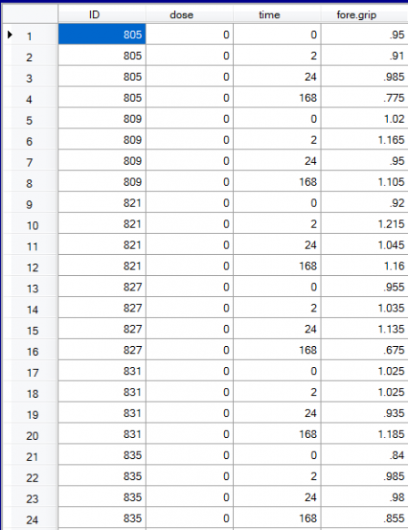
- The response variable measured on a continuous scale.
- A single exposure (or exposure interval) and several (4-5) doses.
- The outcome is measured repeatedly over time on each study subject and the time of observation is given. It is not necessary for each subject to have the same time points.
- The time component is coded between some starting time (usually 0 or 1) and the maximum positive value (last time point for which data is available).
- Individual animal data and multiple subjects per dose group are required.
- Dose effects are observed at more than one dose level, and differences in dose effect are seen at some time points.
- In the Data Grid window, from the Model Type picklist, select Rpt_Resp_Measures. BMDS automatically populates the Model Name field with ToxicoDiffusion.
- Click the Proceed button. BMDS displays a Model Options screen. Edit the fields on the screen so they match the following screenshot and parameters.
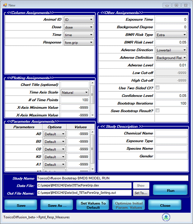
- In the Column Assignments section, use the picklists to select the column name conforming to the label.
- Exposure time = 0
- Background degree = 0
- BMR Risk Type = Extra (EPA recommends extra risk as this accounts for the presence of background responses)
- BMR Risk Level = 0.05 (5% Extra risk)
- Adverse Direction = Lowertail
- Adverse Definition = Background Rate
- Adverse Level = 0.01
-
Click Run to run the model. BMDS will display both text and graphical output (five graphs).
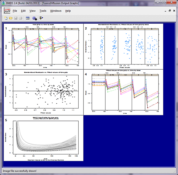
The ToxicoDiffusion model does not produce plot (*.plt) files as do other BMDS models. Instead, these graphs are created in R and saved with an *.emf extension (for “Windows Enhanced Metafile”).
To find the graphic files you created for this exercise, open the BMDS Data subfolder. The .emf file names are a concatenation of the data file name (in this case, TETacForeGrip.dax) with the following suffixes:
| Data File Name | Suffix/Graph Type | Graph File Name |
|---|---|---|
| TETacForeGrip.dax | OT for observed trajectory | TETacForeGripOT.emf |
| TETacForeGrip.dax | ResGBD for residuals grouped by dose | TETacForeGripResGBD.emf |
| TETacForeGrip.dax | Res for residuals for all doses | TETacForeGripRes.emf |
| TETacForeGrip.dax | FT for fitted trajectory | TETacForeGripFT.emf |
| TETacForeGrip.dax | Bstrap for bootstrap | TETacForeGripBStrap.emf |
Double-click on an .emf file to open it in Windows Paint; you can also import it into other graphics viewing or editing programs.
Following are sample images and descriptions of each graph created by the ToxicoDiffusion model.
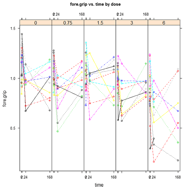 TETacForeGripOT.emf. The Observed Trajectory plot displays each subject’s responses by connecting the observed responses across time. This plot is useful for determining the trajectory of the control group and how exposure changes the trajectory over time.
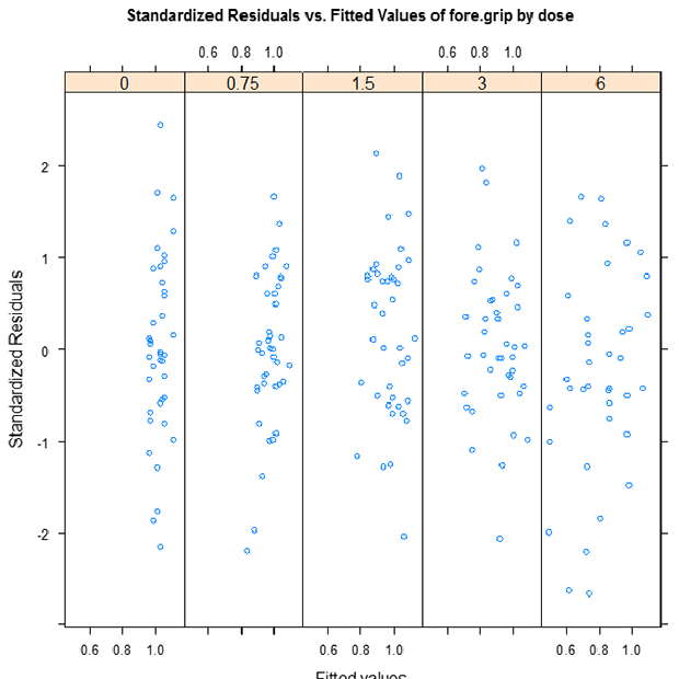 TETacForeGripResGBD.emf. The Pooled Residuals Grouped by Dose plot enables the user to check for randomness in residuals with respect to the level of response within each dose group individually. The presence of any trend (increasing, decreasing, curved) indicates the inappropriateness of the model.
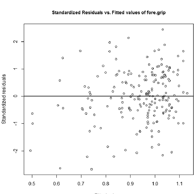 TETacForeGripRes.emf. The Pooled Residuals Across All Dose Groups plot enables the user to check for randomness in residuals with respect to response. The presence of any trend (increasing, decreasing, curved) indicates the inappropriateness of the model.
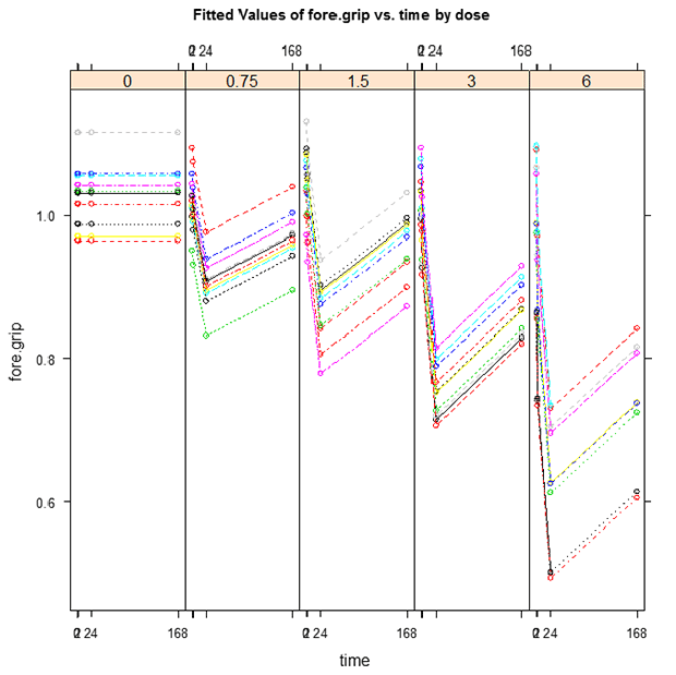 TETacForeGripFT.emf. The Fitted Trajectory plot displays each subject’s fitted responses by connecting the observed responses across time. This plot is useful in determining whether the predicted responses show trajectories resembling the observed trends.
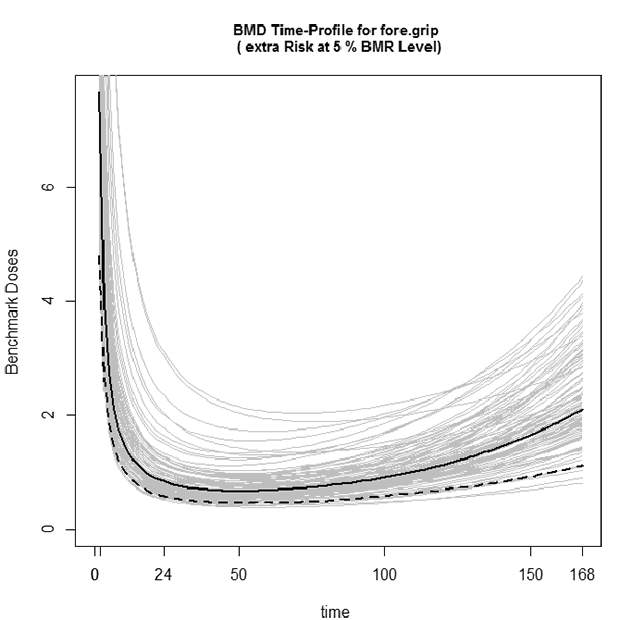 TETacForeGripBStrap.emf. The Bootstrap plot shows the time-profile for each resampled dose-response curve. The bold curve is the original model fit to the data, the light grey curves are the resampled fits, and the dashed bold line represents the fifth percentile of the resampled fits (i.e., this curve corresponds to the 95% lower confidence limit on the original fit).
Questions
- What is the BMDL for the 5% Extra Risk with a 1% Adverse Level, and what test time does this correspond to?
(0.463861. time=50.4)
- From the “Standardized Within-Group Residuals” text output, what are the minimum and maximum within-group residuals? Are these values so extreme as to cause concern over the model fit?
Min=-2.669, Max= 2.446. An absolute value less than 2.5 or 3 can be considered reasonable and not a cause for concern.
- Based on the two residual plots, is there any cause for concern over model fit?
There is no cause for concern. They all look approximately centered at zero with constant spread, and no extreme outliers beyond 3.
- From reviewing the graphs and the text output, do the observed responses in the control group increase or decrease over time?
Overall, decrease. There is a sharp decrease to begin with, followed by an increase in response, with the total direction of effect over the entire test time (from 0 to 168) to be a slight decrease. If you look at the Fitted Trajectory plot, it would appear that the average trend in the control group is no change. In this case, the FT plot is constant for the control dose because the model was run with the background degree = 0. By setting the background degree to 0, we forced the model to assume no change in response.
Exercise 2
In this exercise, you will open and run two different datasets in BMDS and then compare their results.
This exercise explores whether the model fit improves when a parameter is added—in this case, changing the background degree parameter from 0 to 1.
The background degree parameter is an integer between 0 and 2 that determines how the responses are assumed to vary over time in the absence of exposure. This background (without-exposure) variation is defined by a polynomial of the specified degree (constant response=0, linear response=1, or quadratic response=2).
For more information on these model options, refer to the following topic in the BMDS Help file: Using BMDS>Working with the Model Option Screens>Repeated Response Measures Option Screen.
- From within BMDS, select File>Open>Dataset (.dax). Select the file hind_grip.dax and click Open. BMDS displays the file in a new Data Grid window.
- In the Data Grid window, from the Model Type picklist, select Rpt_Resp_Measures. BMDS automatically populates the Model Name field with ToxicoDiffusion.
- Click the Proceed button. BMDS displays a Model Options screen. Make sure the options screen matches the following parameters:
- In the Column Assignments section, use the picklists to select the column name conforming to the label.
- Exposure time = 0
- Background degree = 0
- BMR Risk Type = Extra
- BMR Risk Level = 0.05 (5% Extra risk)
- Adverse Direction = Lowertail
- Adverse Definition = Background Rate
- Adverse Level = 0.05
-
Bootstrap Iterations = 100
- Click Run to run the model. BMDS will display both text and graphical output (five graphs).
- Minimize (do not close) all of the BMDS subwindows (Data Grid, graphs, etc.). You will compare this run’s displays to the second run’s displays.
- Follow Steps 1-3 above, except select a background degree = 1 while leaving all other model parameters as above.
- Arrange the windows so you can compare the text results from both runs side by side.
The following table summarizes the results from the text output of both runs (verify them against your results).
| ToxicoDiffusion (A=0) | ToxicoDiffusion (A=1) | |
|---|---|---|
| Akaike Information Criterion (AIC |
-120.495 | -118.6422 |
| Bayesian Information Criterion (BIC) | -100.7351 | -95.58902 |
| Benchmark Dose (BMD |
0.028027 | 0.028045 |
| Test Time | 28.56 | 28.56 |
| Benchmark Dose-Lower Bound (BMDL |
0.017499 | 0.017276 |
* You may see different BMDL values from those listed in this table. Because the ToxicoDiffusion model uses random bootstrap resampling to calculate the BMDL, the BMDLs calculated from different modeling runs on the same dataset will be slightly different. One way to control this difference is to increase the number of bootstrap iterations, which will decrease the range of calculated BMDLs. For more details on how the model uses bootstrap resampling, refer to page 13 of the ToxicoDiffusion model technical documentation.
Question
- Can you use the Akaike Information Criterion (AIC) and Bayesian Information Criterion (BIC) (which are included in the text report output) to assess whether the addition of an extra parameter improved model fit? Which is the “best” model: A=0 or A=1?
For these two model runs, we’re trying to determine whether adding another parameter affords better fit even when being penalized. In this case it appears that it does not, as the AIC and BIC for A=0 is less than for A=1. Even though visual inspection of the data (by looking at the plots) suggests there is some decrease in response over time in the control group, adding an extra parameter to describe this trend does not increase model fit to a degree to overcome the parameter penalization. In this case, we would choose the A=0 model as the “best” model.
